GLMロジットの影響測定¶

GLMInfluenceのドラフトバージョンに基づいており、これは離散モデル（ロジット、プロビット、ポアソン）にも適用され、最終的には時系列分析以外のほとんどのモデルに拡張される予定です。

ロジスティック回帰の例は、Pregibon (1981年) の「Logistic Regression diagnostics」で使用されており、Finney (1947年) のデータに基づいています。

GLMInfluence は基本的な影響測定を含んでいますが、Pregibon (1981年) で説明されているいくつかの測定、例えば逸脱度や信頼区間への影響に関連する測定はまだ欠けています。

[1]:

import os.path
import pandas as pd
import matplotlib.pyplot as plt

from statsmodels.genmod.generalized_linear_model import GLM
from statsmodels.genmod import families

plt.rc("figure", figsize=(16, 8))
plt.rc("font", size=14)

[2]:

import statsmodels.stats.tests.test_influence

test_module = statsmodels.stats.tests.test_influence.__file__
cur_dir = cur_dir = os.path.abspath(os.path.dirname(test_module))

file_name = "binary_constrict.csv"
file_path = os.path.join(cur_dir, "results", file_name)
df = pd.read_csv(file_path, index_col=0)

[3]:

res = GLM(
    df["constrict"],
    df[["const", "log_rate", "log_volumne"]],
    family=families.Binomial(),
).fit(attach_wls=True, atol=1e-10)
print(res.summary())

                 Generalized Linear Model Regression Results
==============================================================================
Dep. Variable:              constrict   No. Observations:                   39
Model:                            GLM   Df Residuals:                       36
Model Family:                Binomial   Df Model:                            2
Link Function:                  Logit   Scale:                          1.0000
Method:                          IRLS   Log-Likelihood:                -14.614
Date:                Thu, 28 Nov 2024   Deviance:                       29.227
Time:                        23:10:38   Pearson chi2:                     34.2
No. Iterations:                     7   Pseudo R-squ. (CS):             0.4707
Covariance Type:            nonrobust
===============================================================================
                  coef    std err          z      P>|z|      [0.025      0.975]
-------------------------------------------------------------------------------
const          -2.8754      1.321     -2.177      0.029      -5.464      -0.287
log_rate        4.5617      1.838      2.482      0.013       0.959       8.164
log_volumne     5.1793      1.865      2.777      0.005       1.524       8.834
===============================================================================

影響度の測定を取得する¶

GLMResultsにはget_influenceメソッドがあり、これは OLSResults のそれと似たものです。このメソッドは、GLMInfluence クラスのインスタンスを返します。このクラスには、影響度や外れ値の測定を調査するためのメソッドや（キャッシュされた）属性が含まれています。

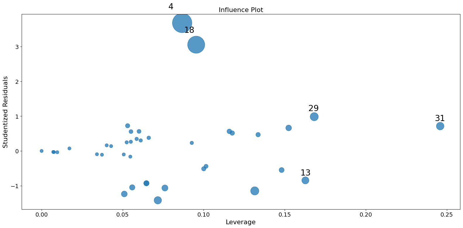
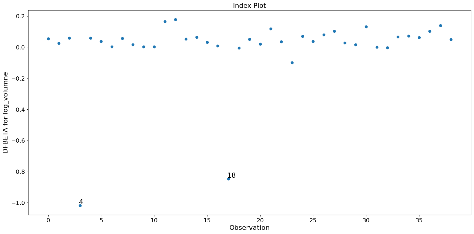
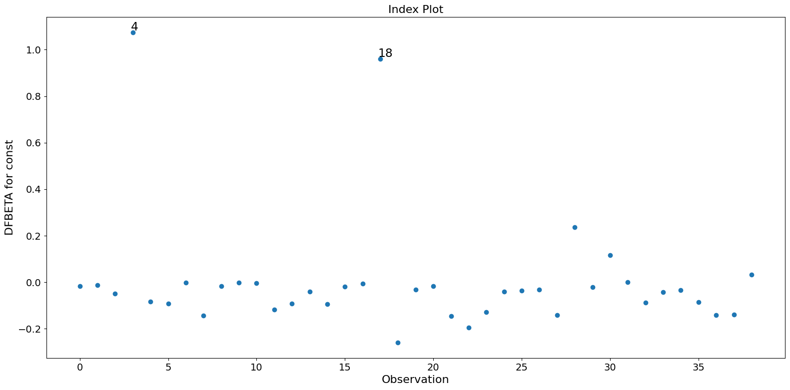
これらの測定は、一つの観測値を削除した場合の結果に対する1ステップ近似に基づいています。1ステップ近似は、小さな変化に対しては通常正確ですが、大きな変化の規模を過小評価する傾向があります。ただし、大きな変化が過小評価されたとしても、影響力のある観測値の効果は明確に示されます。

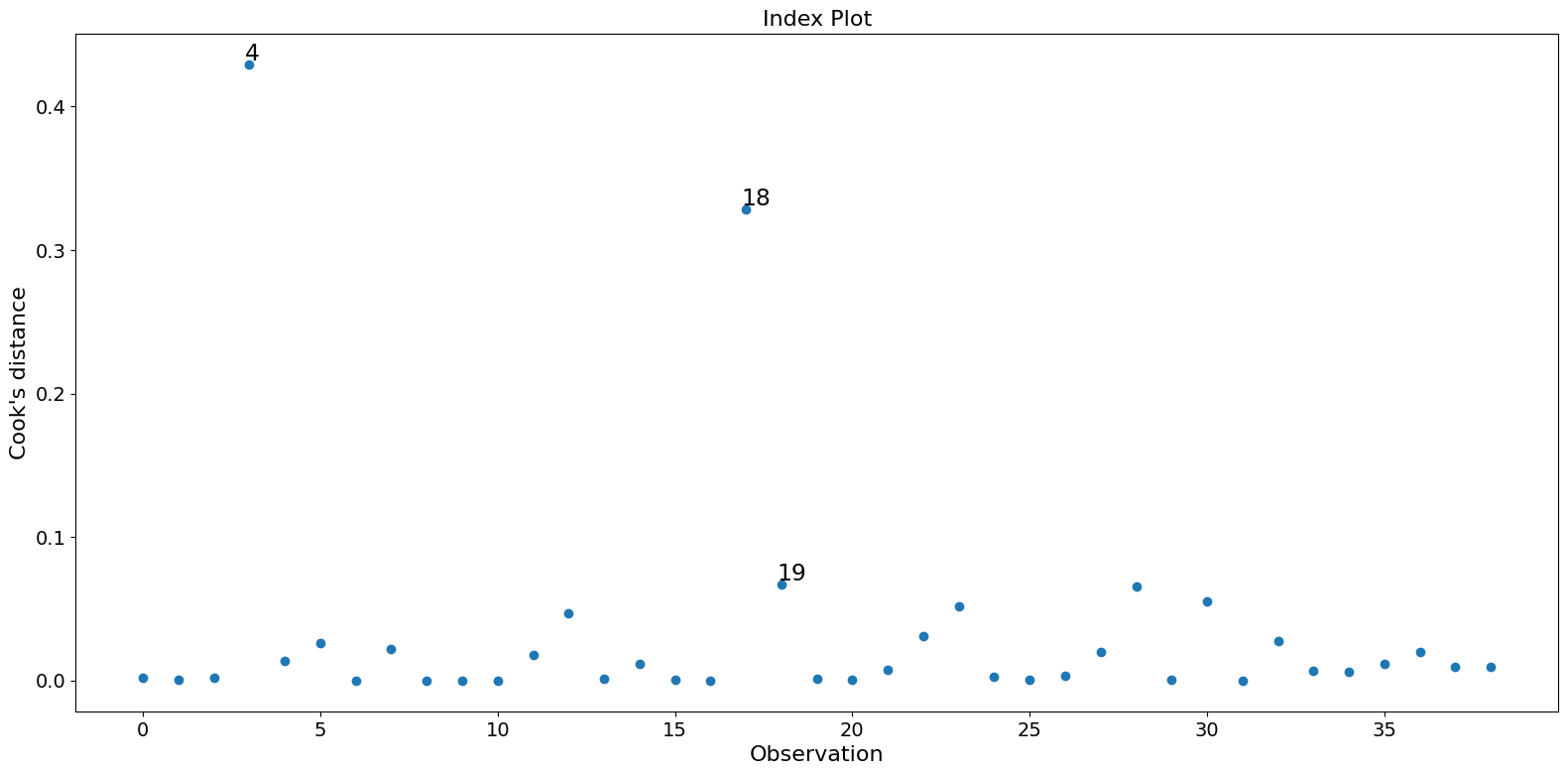
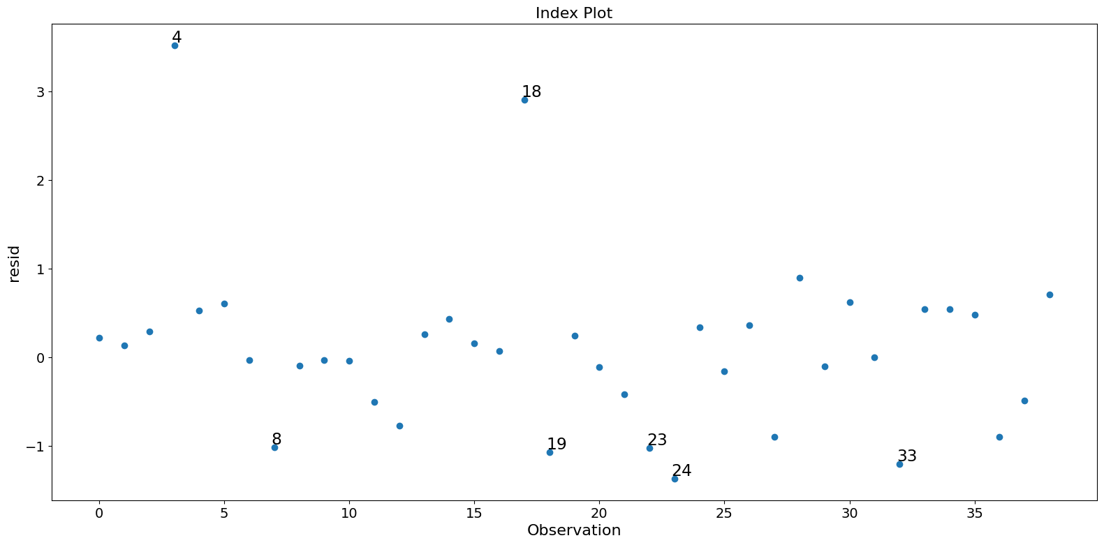
この例では、観測値 4 と 18 が大きな標準化残差と大きなクックの距離を持っていますが、大きなレバレッジはありません。一方で、観測値 13 は最大のレバレッジを持っていますが、クックの距離は小さく、学生化残差も大きくありません。

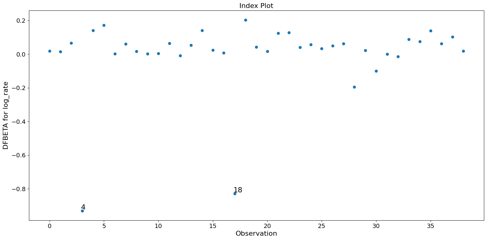
パラメータ推定値に大きな影響を与えるのは、観測値 4 と 18 の二つだけです。

[4]:

infl = res.get_influence(observed=False)

[5]:

summ_df = infl.summary_frame()
summ_df.sort_values("cooks_d", ascending=False)[:10]

[5]:

	dfb_const	dfb_log_rate	dfb_log_volumne	cooks_d	standard_resid	hat_diag	dffits_internal
Case
4	1.073359	-0.930200	-1.017953	0.429085	3.681352	0.086745	1.134573
18	0.959508	-0.827905	-0.847666	0.328152	3.055542	0.095386	0.992197
19	-0.259120	0.202363	-0.004883	0.066770	-1.150095	0.131521	-0.447560
29	0.236747	-0.194984	0.028643	0.065370	0.984729	0.168219	0.442844
31	0.116501	-0.099602	0.132197	0.055382	0.713771	0.245917	0.407609
24	-0.128107	0.041039	-0.100410	0.051950	-1.420261	0.071721	-0.394777
13	-0.093083	-0.009463	0.177532	0.046492	-0.847046	0.162757	-0.373465
23	-0.196119	0.127482	0.035689	0.031168	-1.065576	0.076085	-0.305786
33	-0.088174	-0.013657	-0.002161	0.027481	-1.238185	0.051031	-0.287130
6	-0.092235	0.170980	0.038080	0.026230	0.661478	0.152431	0.280520

[6]:

fig = infl.plot_influence()
fig.tight_layout(pad=1.0)

../../../_images/examples_notebooks_generated_influence_glm_logit_7_0.png

[7]:

fig = infl.plot_index(y_var="cooks", threshold=2 * infl.cooks_distance[0].mean())
fig.tight_layout(pad=1.0)

../../../_images/examples_notebooks_generated_influence_glm_logit_8_0.png

[8]:

fig = infl.plot_index(y_var="resid", threshold=1)
fig.tight_layout(pad=1.0)

../../../_images/examples_notebooks_generated_influence_glm_logit_9_0.png

[9]:

fig = infl.plot_index(y_var="dfbeta", idx=1, threshold=0.5)
fig.tight_layout(pad=1.0)

../../../_images/examples_notebooks_generated_influence_glm_logit_10_0.png

[10]:

fig = infl.plot_index(y_var="dfbeta", idx=2, threshold=0.5)
fig.tight_layout(pad=1.0)

../../../_images/examples_notebooks_generated_influence_glm_logit_11_0.png

[11]:

fig = infl.plot_index(y_var="dfbeta", idx=0, threshold=0.5)
fig.tight_layout(pad=1.0)

../../../_images/examples_notebooks_generated_influence_glm_logit_12_0.png

[ ]:

最終更新日: 2025年01月28日