GEEスコア検定
このノートブックでは、ロバストな GEE スコア検定を示すためにシミュレーションを使用します。これらの検定は、平均構造に関する階層的仮説を比較するためにGEE分析で使用できます。これらの検定は、作業相関モデルの誤指定や、分散構造の特定の誤指定形式(例えば、準ポアソン分析でのスケールパラメータによるもの)に対してロバストです。
データはクラスターとしてシミュレートされ、クラスター内には依存関係がありますが、クラスター間には依存関係はありません。クラスターごとの依存関係は、コピュラアプローチを使用して導入されています。データは、負二項分布(ガンマ/ポアソン)の混合として周辺的に従います。
検定のレベルと検出力については、検定の性能を評価するために以下で考察します。
[1]:
import pandas as pd
import numpy as np
from scipy.stats.distributions import norm, poisson
import statsmodels.api as sm
import matplotlib.pyplot as plt
以下のセルで定義された関数は、コピュラアプローチを使用して、負二項分布に従う相関のあるランダム値をシミュレートします。入力パラメータ u は (0, 1) の範囲の値の配列です。 u の要素は (0, 1) で一様に分布している必要があります。 u の相関は、返される負二項分布の値に相関を生じさせます。配列パラメータ mu は周辺平均を提供し、スカラー値のパラメータ scale は平均と分散の関係を定義します(分散は scale 倍の平均です)。 u と mu の長さは同じでなければなりません。
[2]:
def negbinom(u, mu, scale):
    p = (scale - 1) / scale
    r = mu * (1 - p) / p
    x = np.random.gamma(r, p / (1 - p), len(u))
    return poisson.ppf(u, mu=x)
以下は、シミュレーションで使用されるデータを制御するいくつかのパラメータです。
[3]:
# Sample size
n = 1000

# Number of covariates (including intercept) in the alternative hypothesis model
p = 5

# Cluster size
m = 10

# Intraclass correlation (controls strength of clustering)
r = 0.5

# Group indicators
grp = np.kron(np.arange(n/m), np.ones(m))
シミュレーションでは、固定されたデザイン行列が使用されます。
[4]:
# Build a design matrix for the alternative (more complex) model
x = np.random.normal(size=(n, p))
x[:, 0] = 1
帰無仮説のデザイン行列は、対立仮説のデザイン行列にネストされています。帰無仮説のデザイン行列は、対立仮説のデザイン行列よりランクが2低いです。
[5]:
x0 = x[:, 0:3]
GEE スコア検定は、依存性と過剰分散に対してロバストです。ここでは、過剰分散パラメータを設定します。各観測値に対する負二項分布の分散は、 scale とその平均値を掛け合わせたものに等しくなります。
[6]:
# Scale parameter for negative binomial distribution
scale = 10
次のセルでは、帰無モデルと対立モデルの平均構造を設定します。
[7]:
# The coefficients used to define the linear predictors
coeff = [[4, 0.4, -0.2], [4, 0.4, -0.2, 0, -0.04]]

# The linear predictors
lp = [np.dot(x0, coeff[0]), np.dot(x, coeff[1])]

# The mean values
mu = [np.exp(lp[0]), np.exp(lp[1])]
以下はシミュレーションを実行する関数です。
[8]:
# hyp = 0 is the null hypothesis, hyp = 1 is the alternative hypothesis.
# cov_struct is a statsmodels covariance structure
def dosim(hyp, cov_struct=None, mcrep=500):

    # Storage for the simulation results
    scales = [[], []]

    # P-values from the score test
    pv = []

    # Monte Carlo loop
    for k in range(mcrep):

        # Generate random "probability points" u  that are uniformly
        # distributed, and correlated within clusters
        z = np.random.normal(size=n)
        u = np.random.normal(size=n//m)
        u = np.kron(u, np.ones(m))
        z = r*z +np.sqrt(1-r**2)*u
        u = norm.cdf(z)

        # Generate the observed responses
        y = negbinom(u, mu=mu[hyp], scale=scale)

        # Fit the null model
        m0 = sm.GEE(y, x0, groups=grp, cov_struct=cov_struct, family=sm.families.Poisson())
        r0 = m0.fit(scale='X2')
        scales[0].append(r0.scale)

        # Fit the alternative model
        m1 = sm.GEE(y, x, groups=grp, cov_struct=cov_struct, family=sm.families.Poisson())
        r1 = m1.fit(scale='X2')
        scales[1].append(r1.scale)

        # Carry out the score test
        st = m1.compare_score_test(r0)
        pv.append(st["p-value"])

    pv = np.asarray(pv)
    rslt = [np.mean(pv), np.mean(pv < 0.1)]

    return rslt, scales
独立性を仮定した作業共分散構造を使用してシミュレーションを実行します。帰無仮説の下では平均が約 0 になると予想され、対立仮説の下ではそれよりかなり低くなると予想されます。同様に、帰無仮説の下では p 値の約 10% が 0.1 未満であると予想され、対立仮説の下では p 値が 0.1 未満である割合がはるかに大きくなると予想されます。
[9]:
rslt, scales = [], []

for hyp in 0, 1:
    s, t = dosim(hyp, sm.cov_struct.Independence())
    rslt.append(s)
    scales.append(t)

rslt = pd.DataFrame(rslt, index=["H0", "H1"], columns=["Mean", "Prop(p<0.1)"])

print(rslt)
        Mean  Prop(p<0.1)
H0  0.496915        0.102
H1  0.050089        0.864
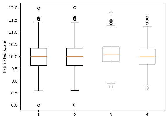
次に、スケールパラメータの推定値が妥当であることを確認します。私たちは GEE スコア検定の依存性と過剰分散に対するロバスト性を評価しているため、ここでは過剰分散が予想通り存在していることを確認しています。
[10]:
_ = plt.boxplot([scales[0][0], scales[0][1], scales[1][0], scales[1][1]])
plt.ylabel("Estimated scale")
[10]:
Text(0, 0.5, 'Estimated scale')
次に、交換可能な作業相関モデルを使用して同じ分析を行います。これは、独立した作業相関を使用した上記の例よりも遅くなるため、モンテカルロの反復回数を少なくします。
[11]:
rslt, scales = [], []

for hyp in 0, 1:
    s, t = dosim(hyp, sm.cov_struct.Exchangeable(), mcrep=100)
    rslt.append(s)
    scales.append(t)

rslt = pd.DataFrame(rslt, index=["H0", "H1"], columns=["Mean", "Prop(p<0.1)"])

print(rslt)
        Mean  Prop(p<0.1)
H0  0.491246         0.08
H1  0.054909         0.86
[ ]:
[ ]: