線形回帰診断
実際のデータでは、応答変数とターゲット変数の関係は線形であることは稀です。ここでは、statsmodelsの出力を使用して、非線形の関係に線形回帰モデルをフィットさせることで発生する可能性のある問題を視覚化し、特定します。主な目的は、Jamesらによる『An Introduction to Statistical Learning』(ISLR)第3.3.3章「Potential Problems」セクションで議論された視覚化を再現することです。
[1]:
import statsmodels
import statsmodels.formula.api as smf
import pandas as pd
単純な重回帰分析
まず、ISLR書籍の第2章から広告データを読み込み、それに線形モデルをフィットさせます。
[2]:
# Load data
data_url = "https://raw.githubusercontent.com/nguyen-toan/ISLR/07fd968ea484b5f6febc7b392a28eb64329a4945/dataset/Advertising.csv"
df = pd.read_csv(data_url).drop('Unnamed: 0', axis=1)
df.head()
[2]:
| TV | Radio | Newspaper | Sales | |
|---|---|---|---|---|
| 0 | 230.1 | 37.8 | 69.2 | 22.1 |
| 1 | 44.5 | 39.3 | 45.1 | 10.4 |
| 2 | 17.2 | 45.9 | 69.3 | 9.3 |
| 3 | 151.5 | 41.3 | 58.5 | 18.5 |
| 4 | 180.8 | 10.8 | 58.4 | 12.9 |
[3]:
# Fitting linear model
res = smf.ols(formula= "Sales ~ TV + Radio + Newspaper", data=df).fit()
res.summary()
[3]:
| Dep. Variable: | Sales | R-squared: | 0.897 |
|---|---|---|---|
| Model: | OLS | Adj. R-squared: | 0.896 |
| Method: | Least Squares | F-statistic: | 570.3 |
| Date: | Thu, 28 Nov 2024 | Prob (F-statistic): | 1.58e-96 |
| Time: | 23:10:43 | Log-Likelihood: | -386.18 |
| No. Observations: | 200 | AIC: | 780.4 |
| Df Residuals: | 196 | BIC: | 793.6 |
| Df Model: | 3 | ||
| Covariance Type: | nonrobust |
| coef | std err | t | P>|t| | [0.025 | 0.975] | |
|---|---|---|---|---|---|---|
| Intercept | 2.9389 | 0.312 | 9.422 | 0.000 | 2.324 | 3.554 |
| TV | 0.0458 | 0.001 | 32.809 | 0.000 | 0.043 | 0.049 |
| Radio | 0.1885 | 0.009 | 21.893 | 0.000 | 0.172 | 0.206 |
| Newspaper | -0.0010 | 0.006 | -0.177 | 0.860 | -0.013 | 0.011 |
| Omnibus: | 60.414 | Durbin-Watson: | 2.084 |
|---|---|---|---|
| Prob(Omnibus): | 0.000 | Jarque-Bera (JB): | 151.241 |
| Skew: | -1.327 | Prob(JB): | 1.44e-33 |
| Kurtosis: | 6.332 | Cond. No. | 454. |
Notes:
[1] Standard Errors assume that the covariance matrix of the errors is correctly specified.
診断図/テーブル
以下に、後で次の診断プロットを生成するために使用する基本コードを示します:
a. 残差
b. QQプロット
c. スケールロケーション
d. レバレッジ
およびテーブル:
a. VIF
[4]:
# base code
import numpy as np
import seaborn as sns
from statsmodels.tools.tools import maybe_unwrap_results
from statsmodels.graphics.gofplots import ProbPlot
from statsmodels.stats.outliers_influence import variance_inflation_factor
import matplotlib.pyplot as plt
from typing import Type


class LinearRegDiagnostic():
    """
    Diagnostic plots to identify potential problems in a linear regression fit.
    Mainly,
        a. non-linearity of data
        b. Correlation of error terms
        c. non-constant variance
        d. outliers
        e. high-leverage points
        f. collinearity

    Authors:
        Prajwal Kafle (p33ajkafle@gmail.com, where 3 = r)
        Does not come with any sort of warranty.
        Please test the code one your end before using.

        Matt Spinelli (m3spinelli@gmail.com, where 3 = r)
        (1) Fixed incorrect annotation of the top most extreme residuals in
            the Residuals vs Fitted and, especially, the Normal Q-Q plots.
        (2) Changed Residuals vs Leverage plot to match closer the y-axis
            range shown in the equivalent plot in the R package ggfortify.
        (3) Added horizontal line at y=0 in Residuals vs Leverage plot to
            match the plots in R package ggfortify and base R.
        (4) Added option for placing a vertical guideline on the Residuals
            vs Leverage plot using the rule of thumb of h = 2p/n to denote
            high leverage (high_leverage_threshold=True).
        (5) Added two more ways to compute the Cook's Distance (D) threshold:
            * 'baseR': D > 1 and D > 0.5 (default)
            * 'convention': D > 4/n
            * 'dof': D > 4 / (n - k - 1)
        (6) Fixed class name to conform to Pascal casing convention
        (7) Fixed Residuals vs Leverage legend to work with loc='best'
    """

    def __init__(self,
                 results: Type[statsmodels.regression.linear_model.RegressionResultsWrapper]) -> None:
        """
        For a linear regression model, generates following diagnostic plots:

        a. residual
        b. qq
        c. scale location and
        d. leverage

        and a table

        e. vif

        Args:
            results (Type[statsmodels.regression.linear_model.RegressionResultsWrapper]):
                must be instance of statsmodels.regression.linear_model object

        Raises:
            TypeError: if instance does not belong to above object

        Example:
        >>> import numpy as np
        >>> import pandas as pd
        >>> import statsmodels.formula.api as smf
        >>> x = np.linspace(-np.pi, np.pi, 100)
        >>> y = 3*x + 8 + np.random.normal(0,1, 100)
        >>> df = pd.DataFrame({'x':x, 'y':y})
        >>> res = smf.ols(formula= "y ~ x", data=df).fit()
        >>> cls = Linear_Reg_Diagnostic(res)
        >>> cls(plot_context="seaborn-v0_8")

        In case you do not need all plots you can also independently make an individual plot/table
        in following ways

        >>> cls = Linear_Reg_Diagnostic(res)
        >>> cls.residual_plot()
        >>> cls.qq_plot()
        >>> cls.scale_location_plot()
        >>> cls.leverage_plot()
        >>> cls.vif_table()
        """

        if isinstance(results, statsmodels.regression.linear_model.RegressionResultsWrapper) is False:
            raise TypeError("result must be instance of statsmodels.regression.linear_model.RegressionResultsWrapper object")

        self.results = maybe_unwrap_results(results)

        self.y_true = self.results.model.endog
        self.y_predict = self.results.fittedvalues
        self.xvar = self.results.model.exog
        self.xvar_names = self.results.model.exog_names

        self.residual = np.array(self.results.resid)
        influence = self.results.get_influence()
        self.residual_norm = influence.resid_studentized_internal
        self.leverage = influence.hat_matrix_diag
        self.cooks_distance = influence.cooks_distance[0]
        self.nparams = len(self.results.params)
        self.nresids = len(self.residual_norm)

    def __call__(self, plot_context='seaborn-v0_8', **kwargs):
        # print(plt.style.available)
        # GH#9157
        if plot_context not in plt.style.available:
            plot_context = 'default'
        with plt.style.context(plot_context):
            fig, ax = plt.subplots(nrows=2, ncols=2, figsize=(10,10))
            self.residual_plot(ax=ax[0,0])
            self.qq_plot(ax=ax[0,1])
            self.scale_location_plot(ax=ax[1,0])
            self.leverage_plot(
                ax=ax[1,1],
                high_leverage_threshold = kwargs.get('high_leverage_threshold'),
                cooks_threshold = kwargs.get('cooks_threshold'))
            plt.show()

        return self.vif_table(), fig, ax,

    def residual_plot(self, ax=None):
        """
        Residual vs Fitted Plot

        Graphical tool to identify non-linearity.
        (Roughly) Horizontal red line is an indicator that the residual has a linear pattern
        """
        if ax is None:
            fig, ax = plt.subplots()

        sns.residplot(
            x=self.y_predict,
            y=self.residual,
            lowess=True,
            scatter_kws={'alpha': 0.5},
            line_kws={'color': 'red', 'lw': 1, 'alpha': 0.8},
            ax=ax)

        # annotations
        residual_abs = np.abs(self.residual)
        abs_resid = np.flip(np.argsort(residual_abs), 0)
        abs_resid_top_3 = abs_resid[:3]
        for i in abs_resid_top_3:
            ax.annotate(
                i,
                xy=(self.y_predict[i], self.residual[i]),
                color='C3')

        ax.set_title('Residuals vs Fitted', fontweight="bold")
        ax.set_xlabel('Fitted values')
        ax.set_ylabel('Residuals')
        return ax

    def qq_plot(self, ax=None):
        """
        Standarized Residual vs Theoretical Quantile plot

        Used to visually check if residuals are normally distributed.
        Points spread along the diagonal line will suggest so.
        """
        if ax is None:
            fig, ax = plt.subplots()

        QQ = ProbPlot(self.residual_norm)
        fig = QQ.qqplot(line='45', alpha=0.5, lw=1, ax=ax)

        # annotations
        abs_norm_resid = np.flip(np.argsort(np.abs(self.residual_norm)), 0)
        abs_norm_resid_top_3 = abs_norm_resid[:3]
        for i, x, y in self.__qq_top_resid(QQ.theoretical_quantiles, abs_norm_resid_top_3):
            ax.annotate(
                i,
                xy=(x, y),
                ha='right',
                color='C3')

        ax.set_title('Normal Q-Q', fontweight="bold")
        ax.set_xlabel('Theoretical Quantiles')
        ax.set_ylabel('Standardized Residuals')
        return ax

    def scale_location_plot(self, ax=None):
        """
        Sqrt(Standarized Residual) vs Fitted values plot

        Used to check homoscedasticity of the residuals.
        Horizontal line will suggest so.
        """
        if ax is None:
            fig, ax = plt.subplots()

        residual_norm_abs_sqrt = np.sqrt(np.abs(self.residual_norm))

        ax.scatter(self.y_predict, residual_norm_abs_sqrt, alpha=0.5);
        sns.regplot(
            x=self.y_predict,
            y=residual_norm_abs_sqrt,
            scatter=False, ci=False,
            lowess=True,
            line_kws={'color': 'red', 'lw': 1, 'alpha': 0.8},
            ax=ax)

        # annotations
        abs_sq_norm_resid = np.flip(np.argsort(residual_norm_abs_sqrt), 0)
        abs_sq_norm_resid_top_3 = abs_sq_norm_resid[:3]
        for i in abs_sq_norm_resid_top_3:
            ax.annotate(
                i,
                xy=(self.y_predict[i], residual_norm_abs_sqrt[i]),
                color='C3')

        ax.set_title('Scale-Location', fontweight="bold")
        ax.set_xlabel('Fitted values')
        ax.set_ylabel(r'$\sqrt{|\mathrm{Standardized\ Residuals}|}$');
        return ax

    def leverage_plot(self, ax=None, high_leverage_threshold=False, cooks_threshold='baseR'):
        """
        Residual vs Leverage plot

        Points falling outside Cook's distance curves are considered observation that can sway the fit
        aka are influential.
        Good to have none outside the curves.
        """
        if ax is None:
            fig, ax = plt.subplots()

        ax.scatter(
            self.leverage,
            self.residual_norm,
            alpha=0.5);

        sns.regplot(
            x=self.leverage,
            y=self.residual_norm,
            scatter=False,
            ci=False,
            lowess=True,
            line_kws={'color': 'red', 'lw': 1, 'alpha': 0.8},
            ax=ax)

        # annotations
        leverage_top_3 = np.flip(np.argsort(self.cooks_distance), 0)[:3]
        for i in leverage_top_3:
            ax.annotate(
                i,
                xy=(self.leverage[i], self.residual_norm[i]),
                color = 'C3')

        factors = []
        if cooks_threshold == 'baseR' or cooks_threshold is None:
            factors = [1, 0.5]
        elif cooks_threshold == 'convention':
            factors = [4/self.nresids]
        elif cooks_threshold == 'dof':
            factors = [4/ (self.nresids - self.nparams)]
        else:
            raise ValueError("threshold_method must be one of the following: 'convention', 'dof', or 'baseR' (default)")
        for i, factor in enumerate(factors):
            label = "Cook's distance" if i == 0 else None
            xtemp, ytemp = self.__cooks_dist_line(factor)
            ax.plot(xtemp, ytemp, label=label, lw=1.25, ls='--', color='red')
            ax.plot(xtemp, np.negative(ytemp), lw=1.25, ls='--', color='red')

        if high_leverage_threshold:
            high_leverage = 2 * self.nparams / self.nresids
            if max(self.leverage) > high_leverage:
                ax.axvline(high_leverage, label='High leverage', ls='-.', color='purple', lw=1)

        ax.axhline(0, ls='dotted', color='black', lw=1.25)
        ax.set_xlim(0, max(self.leverage)+0.01)
        ax.set_ylim(min(self.residual_norm)-0.1, max(self.residual_norm)+0.1)
        ax.set_title('Residuals vs Leverage', fontweight="bold")
        ax.set_xlabel('Leverage')
        ax.set_ylabel('Standardized Residuals')
        plt.legend(loc='best')
        return ax

    def vif_table(self):
        """
        VIF table

        VIF, the variance inflation factor, is a measure of multicollinearity.
        VIF > 5 for a variable indicates that it is highly collinear with the
        other input variables.
        """
        vif_df = pd.DataFrame()
        vif_df["Features"] = self.xvar_names
        vif_df["VIF Factor"] = [variance_inflation_factor(self.xvar, i) for i in range(self.xvar.shape[1])]

        return (vif_df
                .sort_values("VIF Factor")
                .round(2))


    def __cooks_dist_line(self, factor):
        """
        Helper function for plotting Cook's distance curves
        """
        p = self.nparams
        formula = lambda x: np.sqrt((factor * p * (1 - x)) / x)
        x = np.linspace(0.001, max(self.leverage), 50)
        y = formula(x)
        return x, y


    def __qq_top_resid(self, quantiles, top_residual_indices):
        """
        Helper generator function yielding the index and coordinates
        """
        offset = 0
        quant_index = 0
        previous_is_negative = None
        for resid_index in top_residual_indices:
            y = self.residual_norm[resid_index]
            is_negative = y < 0
            if previous_is_negative == None or previous_is_negative == is_negative:
                offset += 1
            else:
                quant_index -= offset
            x = quantiles[quant_index] if is_negative else np.flip(quantiles, 0)[quant_index]
            quant_index += 1
            previous_is_negative = is_negative
            yield resid_index, x, y
上記の広告データに対してフィットさせたモデルと、提供された基本コードを利用して、診断プロットを一つずつ生成します。
[5]:
cls = LinearRegDiagnostic(res)
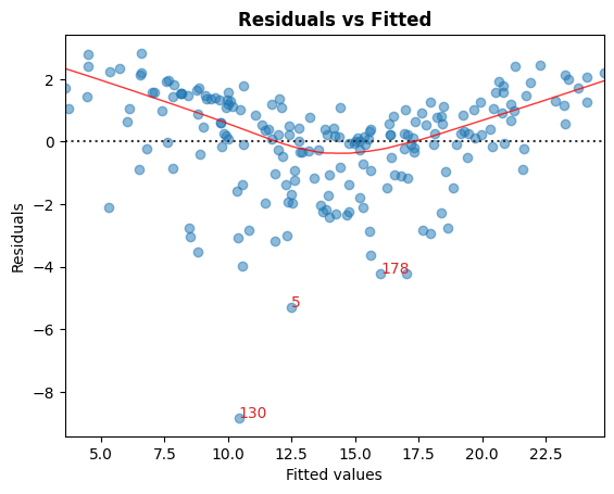
A. 残差とフィット値
非線形性を特定するためのグラフィカルツールです。
グラフにおいて、赤い(おおよそ)水平線は、残差に線形のパターンがあることを示す指標です。
[6]:
cls.residual_plot();
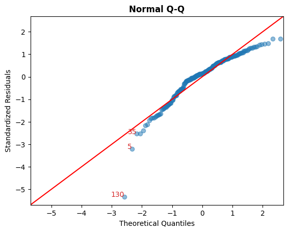
B. 標準化残差と理論的分位数
このプロットは、残差が正規分布しているかを視覚的に確認するために使用されます。
対角線上に沿って点が広がっている場合、それを示唆するものとなります。
[7]:
cls.qq_plot();
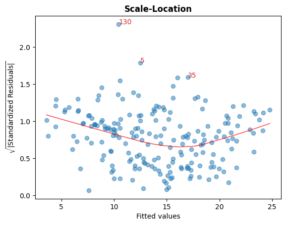
C. 標準化残差の平方根 vs フィッティング値
このプロットは、残差の等分散性(ホモスケダスティシティ)を確認するために使用されます。
グラフ内にほぼ水平な赤い線が表示されている場合、それは等分散性を示唆しています。
[8]:
cls.scale_location_plot();
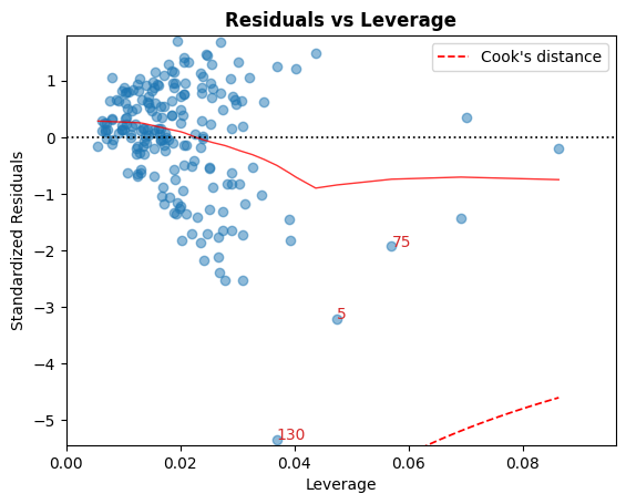
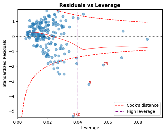
D. 残差 vs レバレッジ
クック距離の曲線の外に位置する点は、フィッティングを左右する可能性がある観測値、すなわち影響力のある観測値と見なされます。
これらの曲線の外に点がないことが望ましいです。
[9]:
cls.leverage_plot();
Cookの距離曲線は、他の経験則を使用して描くことができます:
経験則 |
閾値(s) |
|---|---|
|
\[D_i > 1 \mid D_i > 0.5\]
|
|
\[D_i > { 4 \over n}\]
|
|
\[D_i > {4 \over n - k - 1}\]
|
高いレバレッジのガイドラインは、次のように表示することもできます:\(h_{ii} > {2p \over n}\)。
[10]:
cls.leverage_plot(high_leverage_threshold=True, cooks_threshold='dof');
E. VIF
分散膨張係数(VIF)は、多重共線性の指標です。
ある変数の VIF が 5 を超える場合、その変数は他の入力変数と高い共線性があることを示しています。
[11]:
cls.vif_table()
[11]:
| Features | VIF Factor | |
|---|---|---|
| 1 | TV | 1.00 |
| 2 | Radio | 1.14 |
| 3 | Newspaper | 1.15 |
| 0 | Intercept | 6.85 |
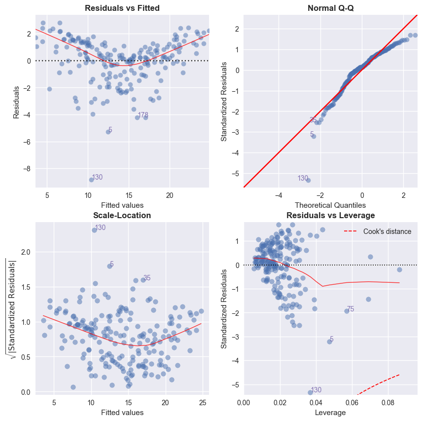
[12]:
# Alternatively, all diagnostics can be generated in one go as follows.
# Fig and ax can be used to modify axes or plot properties after the fact.
cls = LinearRegDiagnostic(res)
vif, fig, ax = cls()
print(vif)

#fig.savefig('../../docs/source/_static/images/linear_regression_diagnostics_plots.png')
    Features  VIF Factor
1         TV        1.00
2      Radio        1.14
3  Newspaper        1.15
0  Intercept        6.85
上記のグラフの解釈と注意事項に関する詳細な説明については、ISLR ブックを参照してください。