回帰プロット
[1]:
%matplotlib inline
[2]:
from statsmodels.compat import lzip
import numpy as np
import matplotlib.pyplot as plt
import statsmodels.api as sm
from statsmodels.formula.api import ols

plt.rc("figure", figsize=(16, 8))
plt.rc("font", size=14)
ダンカンの職業名声データセット
データをロードする
私たちは、優れた Rdatasetsパッケージ から利用可能な任意のRデータセットをロードするためのユーティリティ関数を使用できます。
[3]:
prestige = sm.datasets.get_rdataset("Duncan", "carData", cache=True).data
[4]:
prestige.head()
[4]:
| type | income | education | prestige | |
|---|---|---|---|---|
| rownames | ||||
| accountant | prof | 62 | 86 | 82 |
| pilot | prof | 72 | 76 | 83 |
| architect | prof | 75 | 92 | 90 |
| author | prof | 55 | 90 | 76 |
| chemist | prof | 64 | 86 | 90 |
[5]:
prestige_model = ols("prestige ~ income + education", data=prestige).fit()
[6]:
print(prestige_model.summary())
                            OLS Regression Results
==============================================================================
Dep. Variable:               prestige   R-squared:                       0.828
Model:                            OLS   Adj. R-squared:                  0.820
Method:                 Least Squares   F-statistic:                     101.2
Date:                Wed, 28 Aug 2024   Prob (F-statistic):           8.65e-17
Time:                        14:31:08   Log-Likelihood:                -178.98
No. Observations:                  45   AIC:                             364.0
Df Residuals:                      42   BIC:                             369.4
Df Model:                           2
Covariance Type:            nonrobust
==============================================================================
                 coef    std err          t      P>|t|      [0.025      0.975]
------------------------------------------------------------------------------
Intercept     -6.0647      4.272     -1.420      0.163     -14.686       2.556
income         0.5987      0.120      5.003      0.000       0.357       0.840
education      0.5458      0.098      5.555      0.000       0.348       0.744
==============================================================================
Omnibus:                        1.279   Durbin-Watson:                   1.458
Prob(Omnibus):                  0.528   Jarque-Bera (JB):                0.520
Skew:                           0.155   Prob(JB):                        0.771
Kurtosis:                       3.426   Cond. No.                         163.
==============================================================================

Notes:
[1] Standard Errors assume that the covariance matrix of the errors is correctly specified.
影響度プロット
影響度プロットは、ハット行列によって測定された各観測値のレバレッジに対する(外部の)スチューデント化残差を示します。
外部スチューデント化残差は、標準偏差でスケールされた残差であり、次のように定義されます。
ここで、
\(n\) は観測数、\(p\) は回帰変数の数です。\(h_{ii}\) はハット行列の\(i\)番目の対角要素で、次のように計算されます。
各データ点の影響は、criterionキーワード引数を使用して視覚化できます。オプションとして、影響を測定する2つの指標であるクックの距離(Cook’s distance)とDFFITSがあります。
[7]:
fig = sm.graphics.influence_plot(prestige_model, criterion="cooks")
fig.tight_layout(pad=1.0)
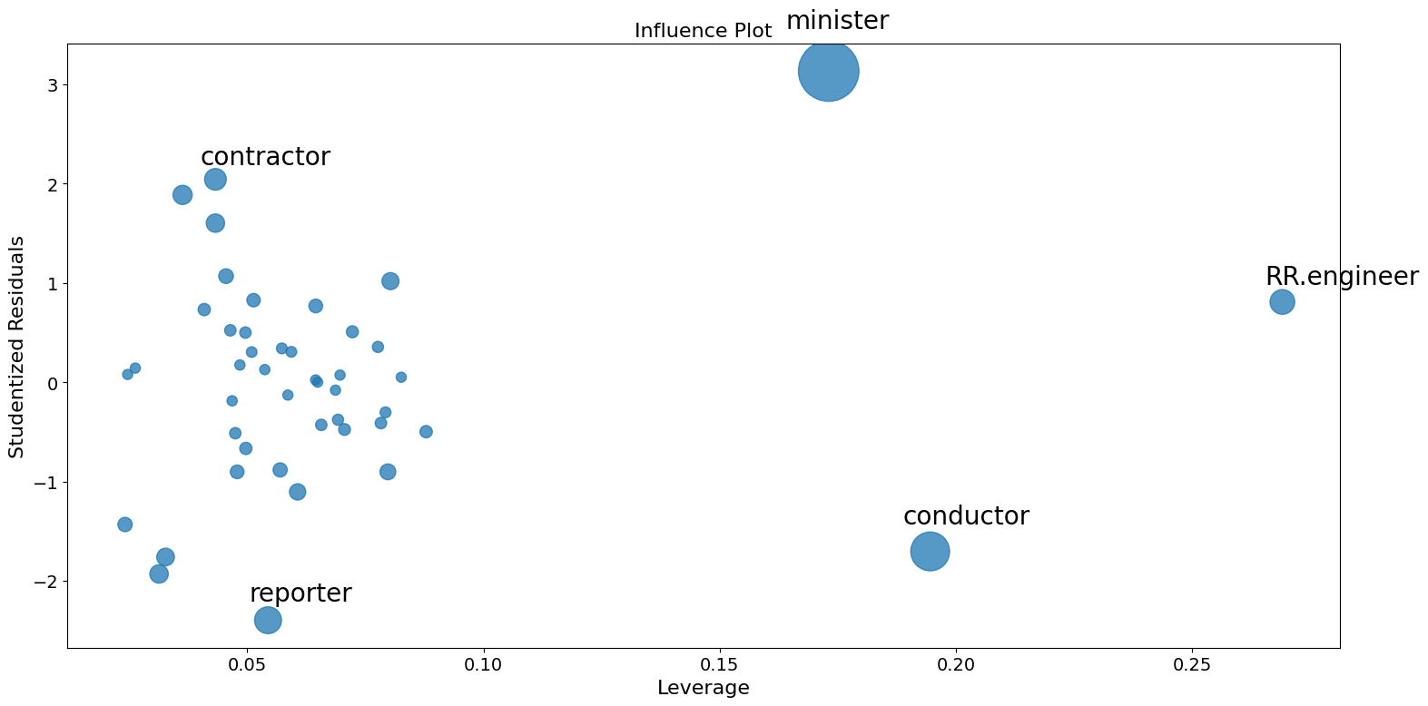
ご覧のとおり、いくつか気になる点があります。請負業者(contractor)と記者(reporter)はどちらもレバレッジは低いですが、残差は大きいです。鉄道技師(RR.engineer) は残差は小さいですが、レバレッジは大きいです。経営者(conductor)と聖職者(ministor)はどちらもレバレッジが高く、残差も大きいため、影響力も大きいです。
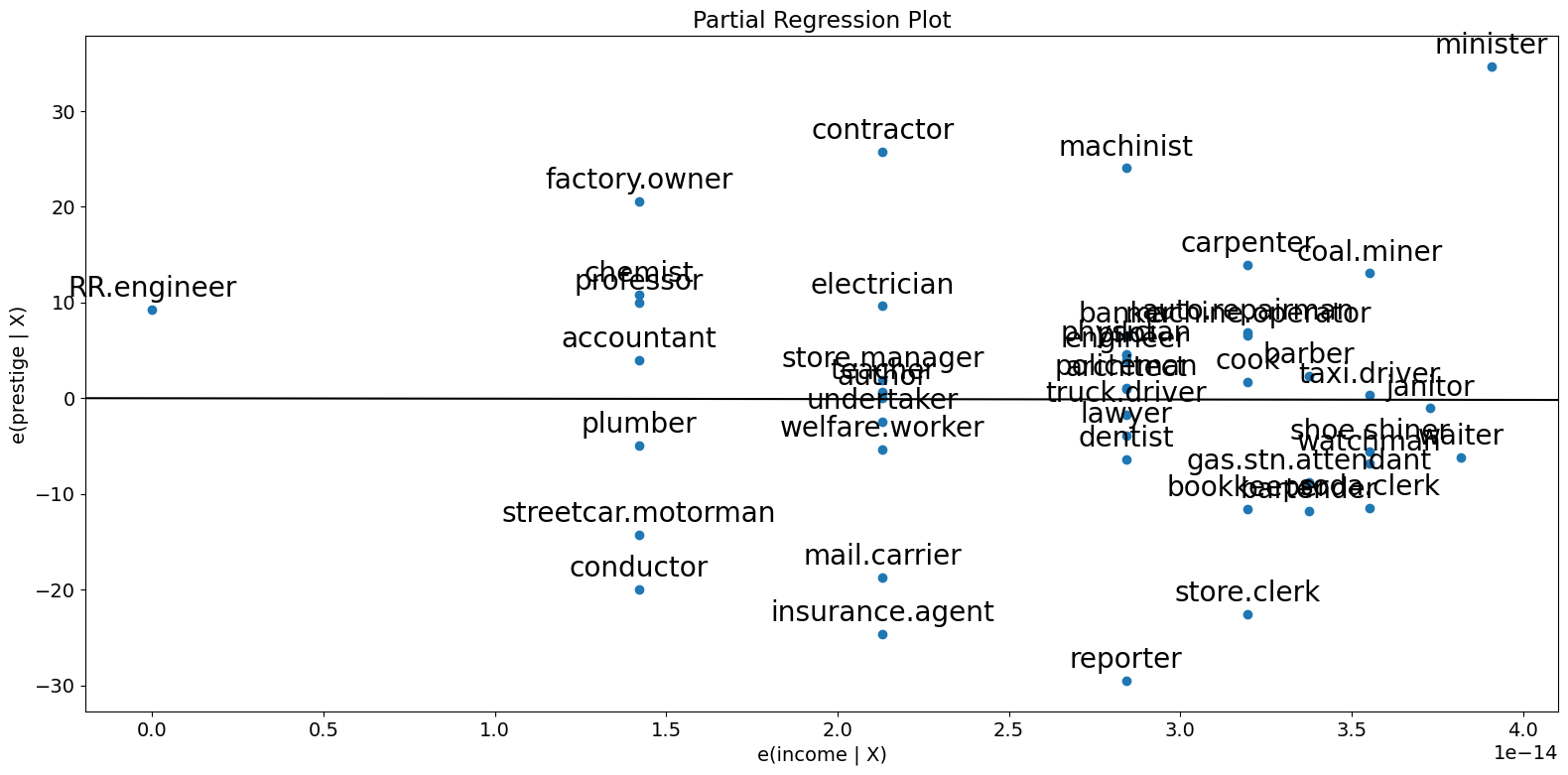
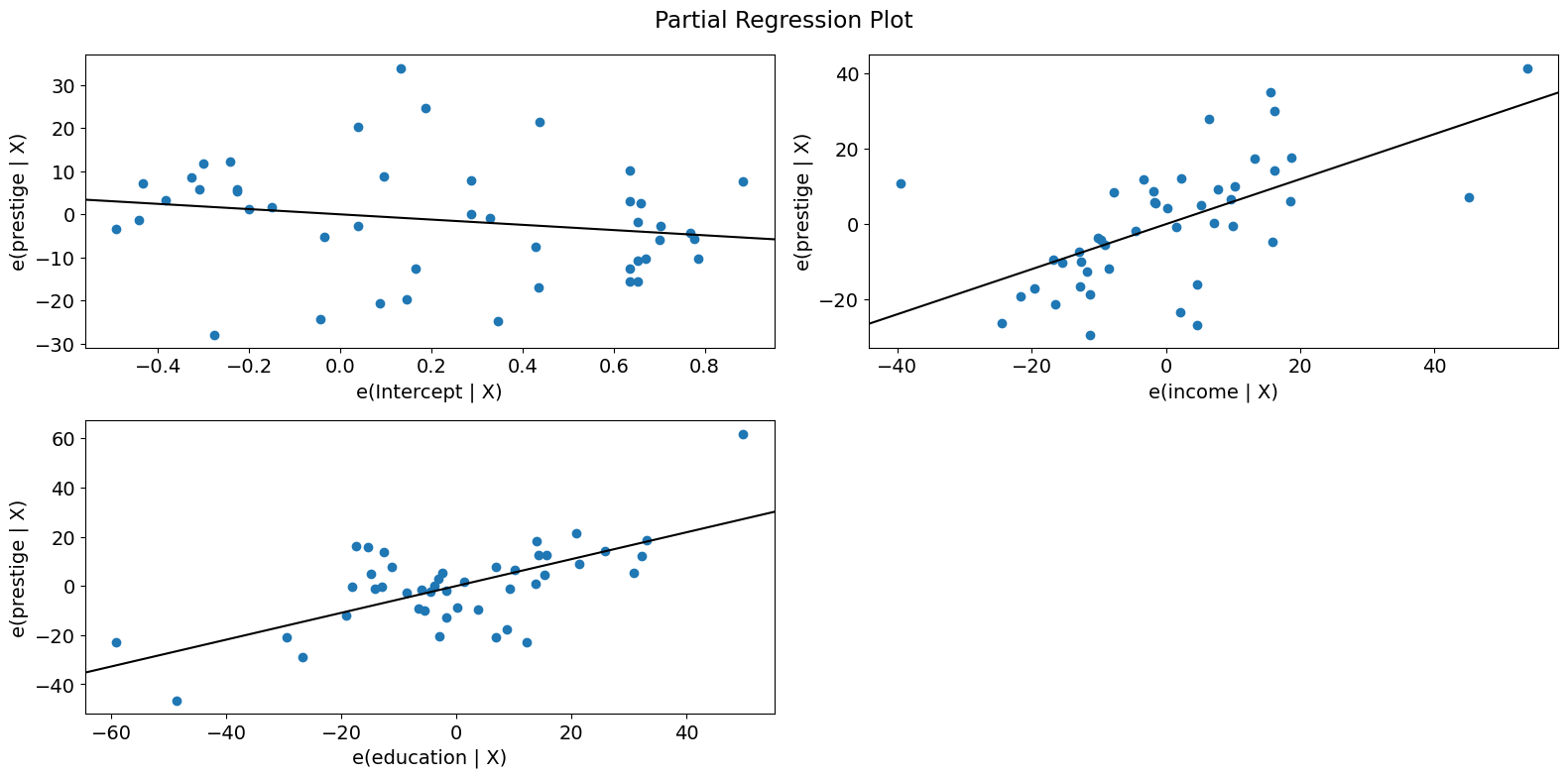
偏回帰プロット (ダンカン)
多変量回帰を行っているため、個々の2変量プロットだけを見て関係を判断することはできません。 代わりに、他の独立変数を条件にした従属変数と独立変数の関係を見たいと考えています。 これを部分回帰プロット(別名:追加変数プロット)を使用して行うことができます。
部分回帰プロットでは、応答変数と\(k\)番目の変数との関係を判別するために、 応答変数を\(X_k\)を除く独立変数に対して回帰させて残差を計算します。これを\(X_{\sim k}\)と表記できます。 次に、\(X_{\sim k}\)に対して\(X_k\)を回帰させて残差を計算します。部分回帰プロットは、前者と後者の残差のプロットです。
このプロットの注目すべき点は、フィットした直線の傾きが\(\beta_k\)であり、切片がゼロであることです。このプロットの残差は、 元のモデルの最小二乗フィットと同じです。係数の推定に対する個別のデータ値の影響を簡単に判別できます。 もしobs_labelsがTrueであれば、これらの点には観測ラベルが注釈として付けられます。また、 等分散性や線形性といった基礎となる仮定の違反も確認できます。
[8]:
fig = sm.graphics.plot_partregress(
    "prestige", "income", ["income", "education"], data=prestige
)
fig.tight_layout(pad=1.0)
[9]:
fig = sm.graphics.plot_partregress("prestige", "income", ["education"], data=prestige)
fig.tight_layout(pad=1.0)
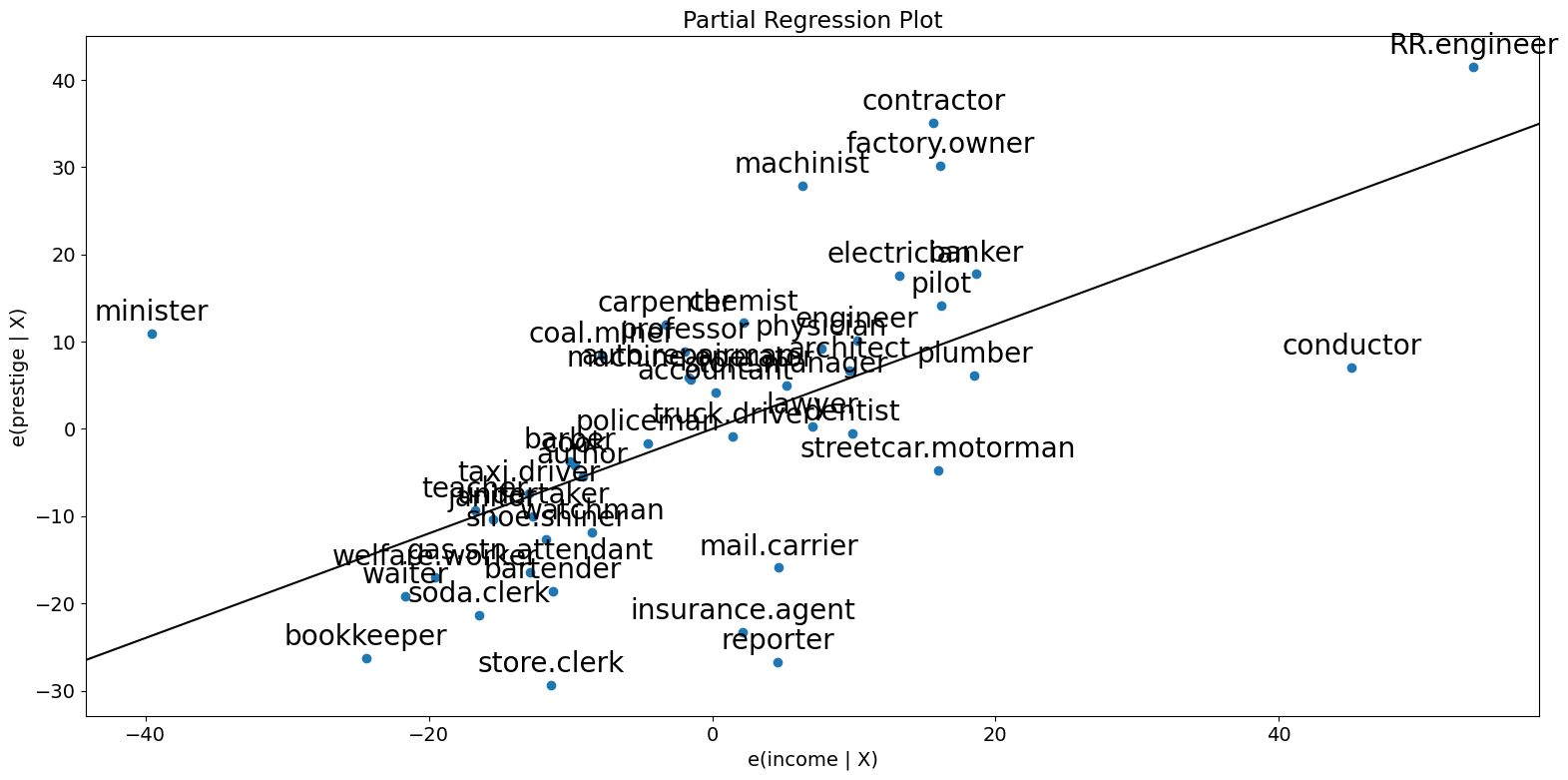
ご覧のように、偏回帰プロットは、収入と名声の部分的な関係に対する経営者(conductor,)者、聖職者(minister,)、鉄道技師(RR.engineer)の影響を確認しています。これらの事例は、収入が名声に及ぼす影響を大幅に減少させます。これらの事例を削除すると、これが確認されます。
[10]:
subset = ~prestige.index.isin(["conductor", "RR.engineer", "minister"])
prestige_model2 = ols(
    "prestige ~ income + education", data=prestige, subset=subset
).fit()
print(prestige_model2.summary())
                            OLS Regression Results
==============================================================================
Dep. Variable:               prestige   R-squared:                       0.876
Model:                            OLS   Adj. R-squared:                  0.870
Method:                 Least Squares   F-statistic:                     138.1
Date:                Wed, 28 Aug 2024   Prob (F-statistic):           2.02e-18
Time:                        14:31:09   Log-Likelihood:                -160.59
No. Observations:                  42   AIC:                             327.2
Df Residuals:                      39   BIC:                             332.4
Df Model:                           2
Covariance Type:            nonrobust
==============================================================================
                 coef    std err          t      P>|t|      [0.025      0.975]
------------------------------------------------------------------------------
Intercept     -6.3174      3.680     -1.717      0.094     -13.760       1.125
income         0.9307      0.154      6.053      0.000       0.620       1.242
education      0.2846      0.121      2.345      0.024       0.039       0.530
==============================================================================
Omnibus:                        3.811   Durbin-Watson:                   1.468
Prob(Omnibus):                  0.149   Jarque-Bera (JB):                2.802
Skew:                          -0.614   Prob(JB):                        0.246
Kurtosis:                       3.303   Cond. No.                         158.
==============================================================================

Notes:
[1] Standard Errors assume that the covariance matrix of the errors is correctly specified.
すべての回帰変数を簡単にチェックするには、 plot_partregress_grid を使用します。これらのプロットはポイントにラベルを付けませんが、問題を特定するために使用した後で、plot_partregress を使用して詳細情報を取得できます。
[11]:
fig = sm.graphics.plot_partregress_grid(prestige_model)
fig.tight_layout(pad=1.0)
成分-成分+残差(CCPR)プロット
CCPR プロットは、他の独立変数の影響を考慮に入れた上で、1つの回帰変数が応答変数に与える影響を判断する方法を提供します。部分残差プロットは、\(\text{残差} + B_iX_i\) を \(X_i\) に対してプロットしたものとして定義されます。この成分は、\(B_iX_i\) と \(X_i\) を対比させて、適合した直線がどこに位置するかを示します。もし \(X_i\) が他の独立変数のいずれかと高い相関を持つ場合には注意が必要です。この場合、プロットに現れる分散は、真の分散を過小評価したものになります。
[12]:
fig = sm.graphics.plot_ccpr(prestige_model, "education")
fig.tight_layout(pad=1.0)
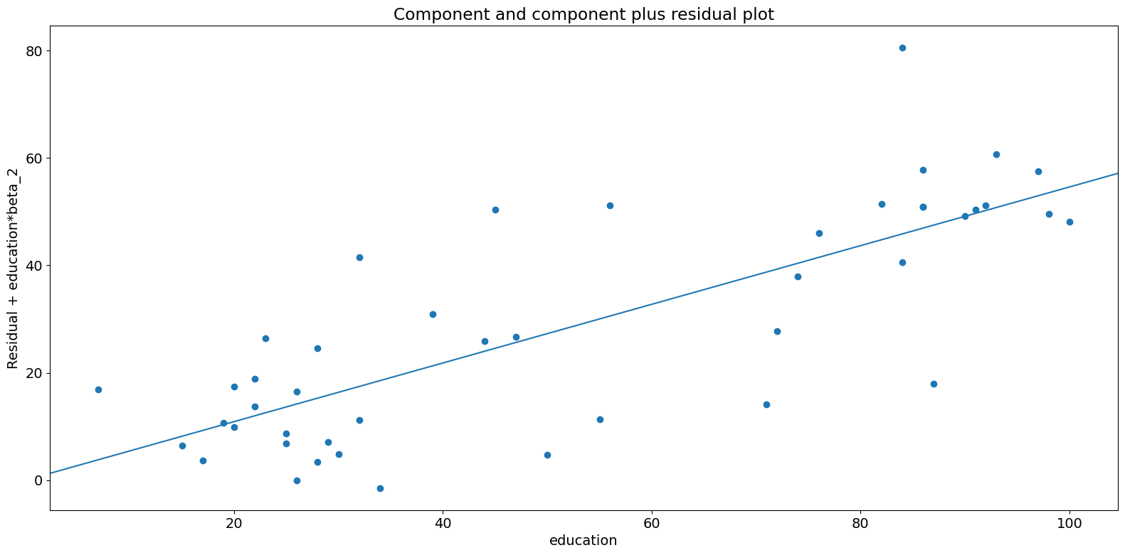
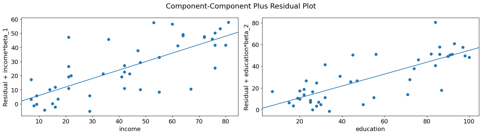
このように、収入を条件とした教育によって説明される名声の変動の間の関係は、直線的であるように見えますが、この関係にかなりの影響を及ぼしているいくつかの観察結果があることがわかります。plot_ccpr_grid を使用すると、複数の変数をすばやく調べることができます。
[13]:
fig = sm.graphics.plot_ccpr_grid(prestige_model)
fig.tight_layout(pad=1.0)
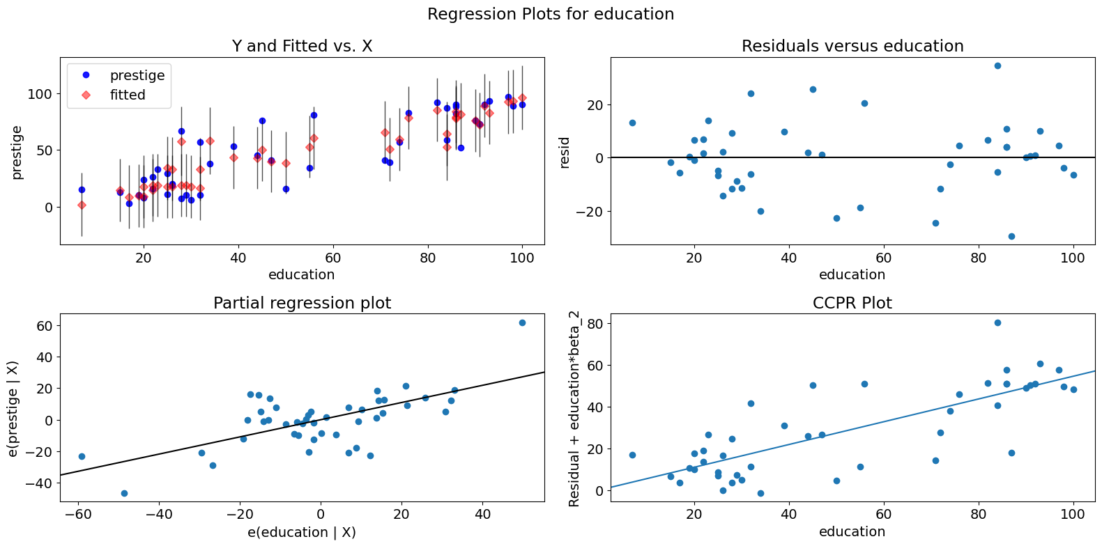
単変数回帰診断
plot_regress_exog 関数は、選択した独立変数に対する信頼区間、選択した独立変数に対するモデルの残差、部分回帰プロット、および CCPR プロットを含む 2x2 プロットを提供する便利な関数です。この関数は、単一の回帰変数に関するモデリングの仮定をすばやくチェックするために使用できます。
[14]:
fig = sm.graphics.plot_regress_exog(prestige_model, "education")
fig.tight_layout(pad=1.0)
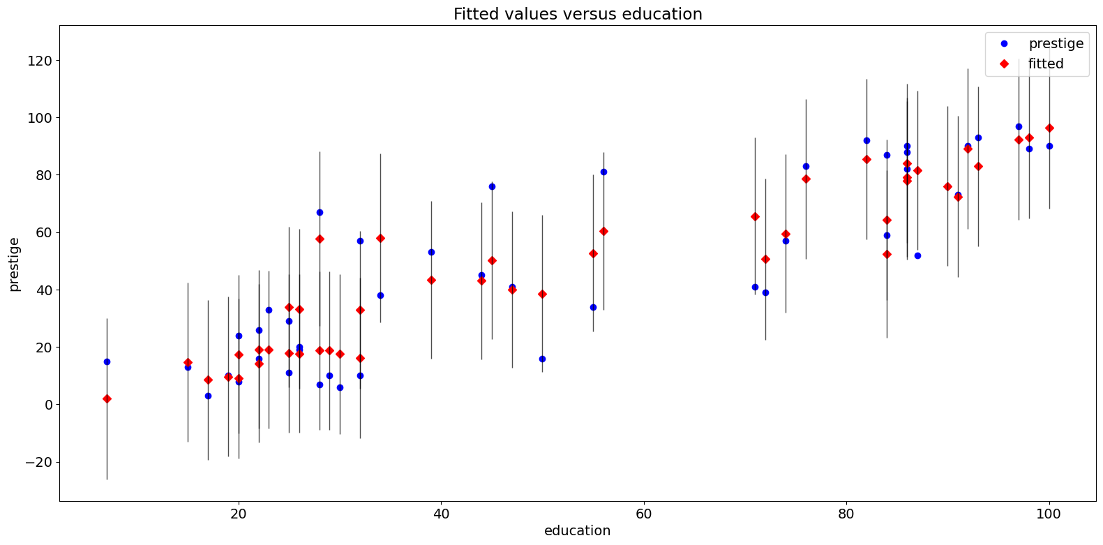
適合度プロット
plot_fit 関数は、選択した独立変数に対してフィットした値をプロットします。これには予測信頼区間が含まれ、オプションで真の従属変数がプロットされます。
[15]:
fig = sm.graphics.plot_fit(prestige_model, "education")
fig.tight_layout(pad=1.0)
2009年 州犯罪データセット
以下を http://www.ats.ucla.edu/stat/stata/webbooks/reg/chapter4/statareg_self_assessment_answers4.htm と比較します。
ただし、ここで使用するデータはその例のものとは異なります。必要なセルのコメントを外すことで、その例を実行することができます。
(翻訳者注:上記参照先はリンクが切れています。元のコースドキュメントは以下のURLの文中のChapter4と思われるので参考まで掲載しておきます。 https://stats.oarc.ucla.edu/stata/webbooks/reg/stata-web-books-regression-with-stata/ )
[16]:
# dta = pd.read_csv("http://www.stat.ufl.edu/~aa/social/csv_files/statewide-crime-2.csv")
# dta = dta.set_index("State", inplace=True).dropna()
# dta.rename(columns={"VR" : "crime",
#                    "MR" : "murder",
#                    "M"  : "pctmetro",
#                    "W"  : "pctwhite",
#                    "H"  : "pcths",
#                    "P"  : "poverty",
#                    "S"  : "single"
#                    }, inplace=True)
#
# crime_model = ols("murder ~ pctmetro + poverty + pcths + single", data=dta).fit()
[17]:
dta = sm.datasets.statecrime.load_pandas().data
[18]:
crime_model = ols("murder ~ urban + poverty + hs_grad + single", data=dta).fit()
print(crime_model.summary())
                            OLS Regression Results
==============================================================================
Dep. Variable:                 murder   R-squared:                       0.813
Model:                            OLS   Adj. R-squared:                  0.797
Method:                 Least Squares   F-statistic:                     50.08
Date:                Wed, 28 Aug 2024   Prob (F-statistic):           3.42e-16
Time:                        14:31:11   Log-Likelihood:                -95.050
No. Observations:                  51   AIC:                             200.1
Df Residuals:                      46   BIC:                             209.8
Df Model:                           4
Covariance Type:            nonrobust
==============================================================================
                 coef    std err          t      P>|t|      [0.025      0.975]
------------------------------------------------------------------------------
Intercept    -44.1024     12.086     -3.649      0.001     -68.430     -19.774
urban          0.0109      0.015      0.707      0.483      -0.020       0.042
poverty        0.4121      0.140      2.939      0.005       0.130       0.694
hs_grad        0.3059      0.117      2.611      0.012       0.070       0.542
single         0.6374      0.070      9.065      0.000       0.496       0.779
==============================================================================
Omnibus:                        1.618   Durbin-Watson:                   2.507
Prob(Omnibus):                  0.445   Jarque-Bera (JB):                0.831
Skew:                          -0.220   Prob(JB):                        0.660
Kurtosis:                       3.445   Cond. No.                     5.80e+03
==============================================================================

Notes:
[1] Standard Errors assume that the covariance matrix of the errors is correctly specified.
[2] The condition number is large, 5.8e+03. This might indicate that there are
strong multicollinearity or other numerical problems.
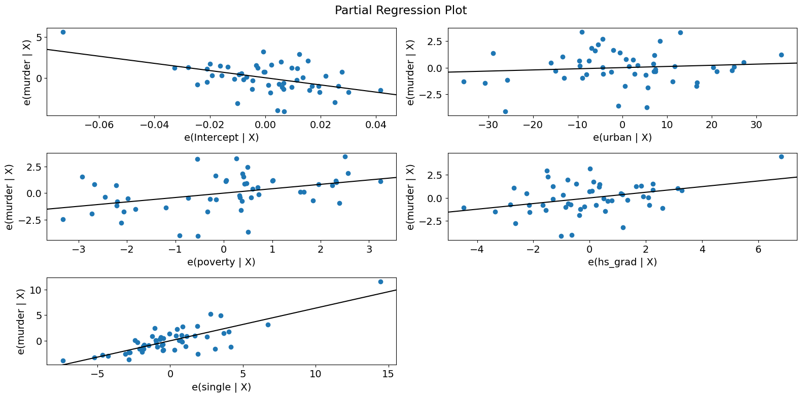
偏回帰プロット(犯罪データ)
[19]:
fig = sm.graphics.plot_partregress_grid(crime_model)
fig.tight_layout(pad=1.0)
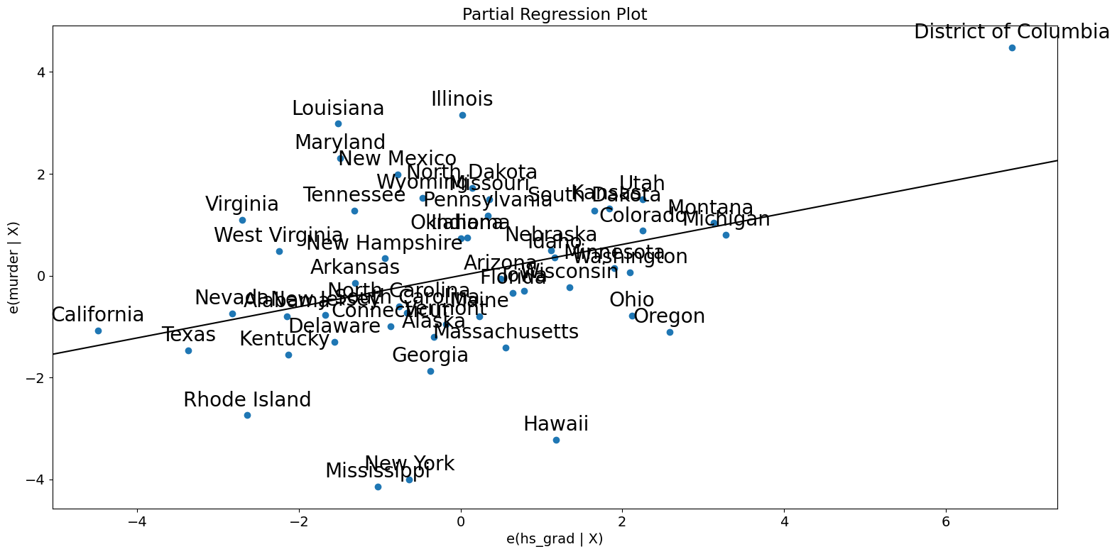
[20]:
fig = sm.graphics.plot_partregress(
    "murder", "hs_grad", ["urban", "poverty", "single"], data=dta
)
fig.tight_layout(pad=1.0)
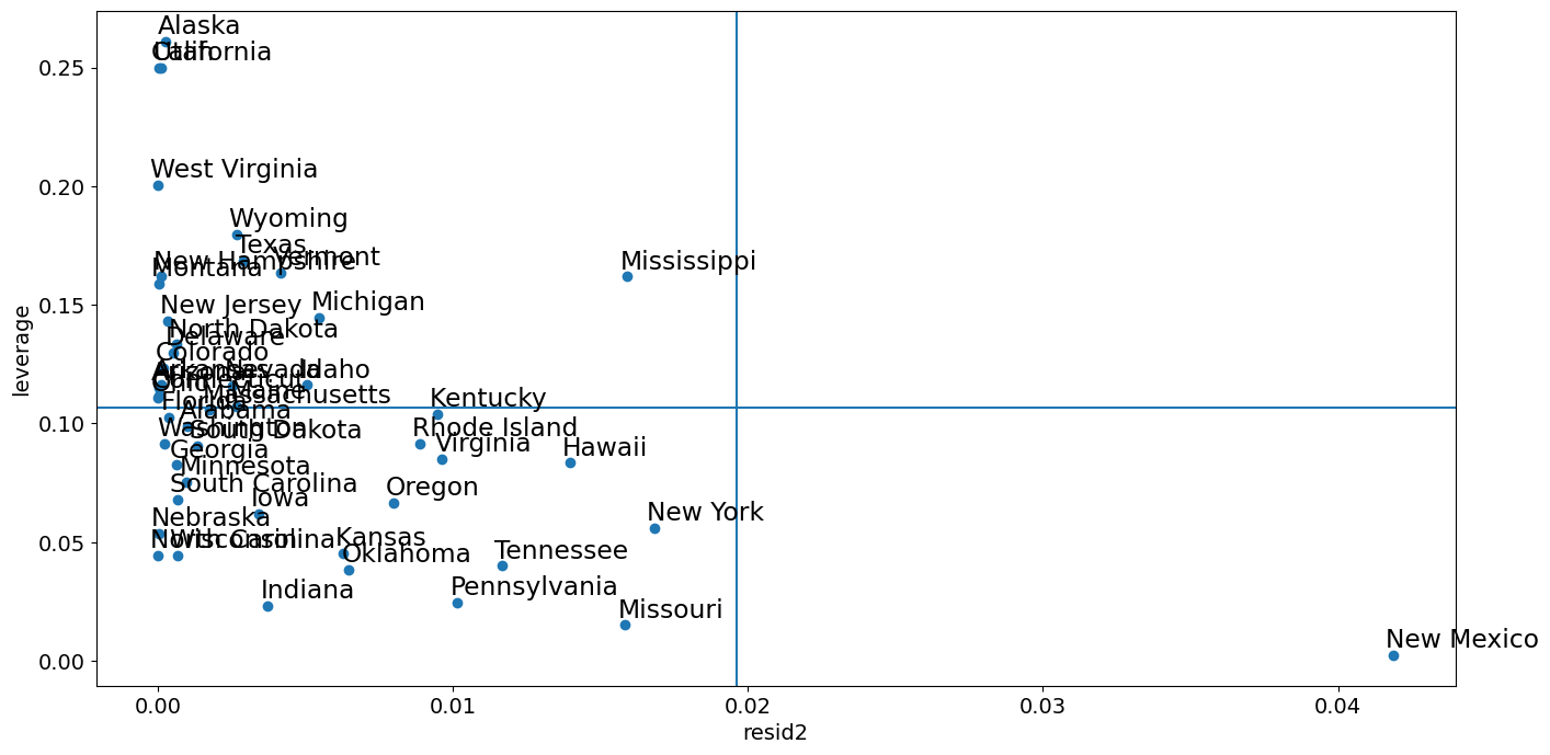
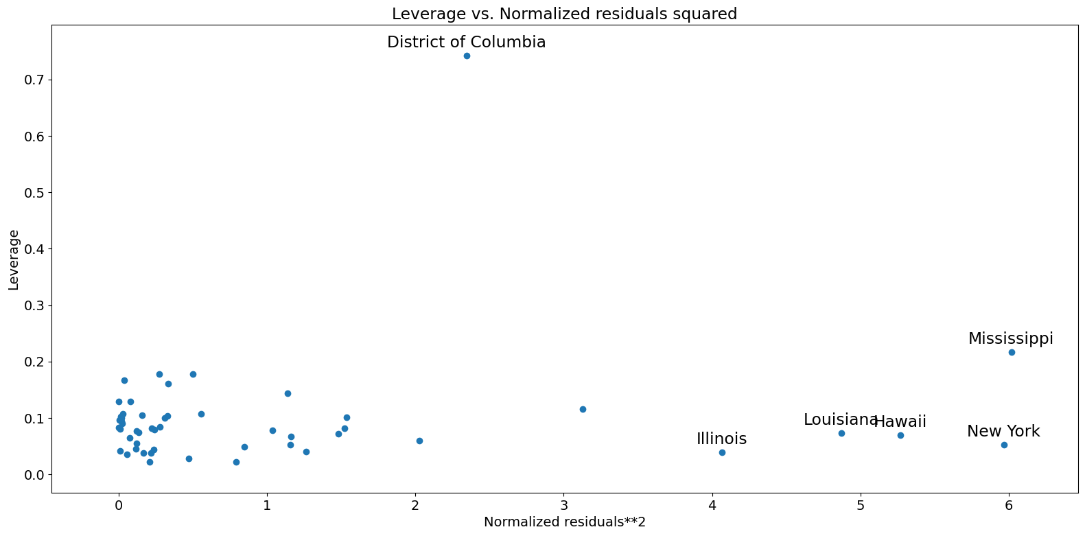
レバレッジ-残差2プロット
「influence_plot」に密接に関連しているのが、leverage-resid2プロットです。
[21]:
fig = sm.graphics.plot_leverage_resid2(crime_model)
fig.tight_layout(pad=1.0)
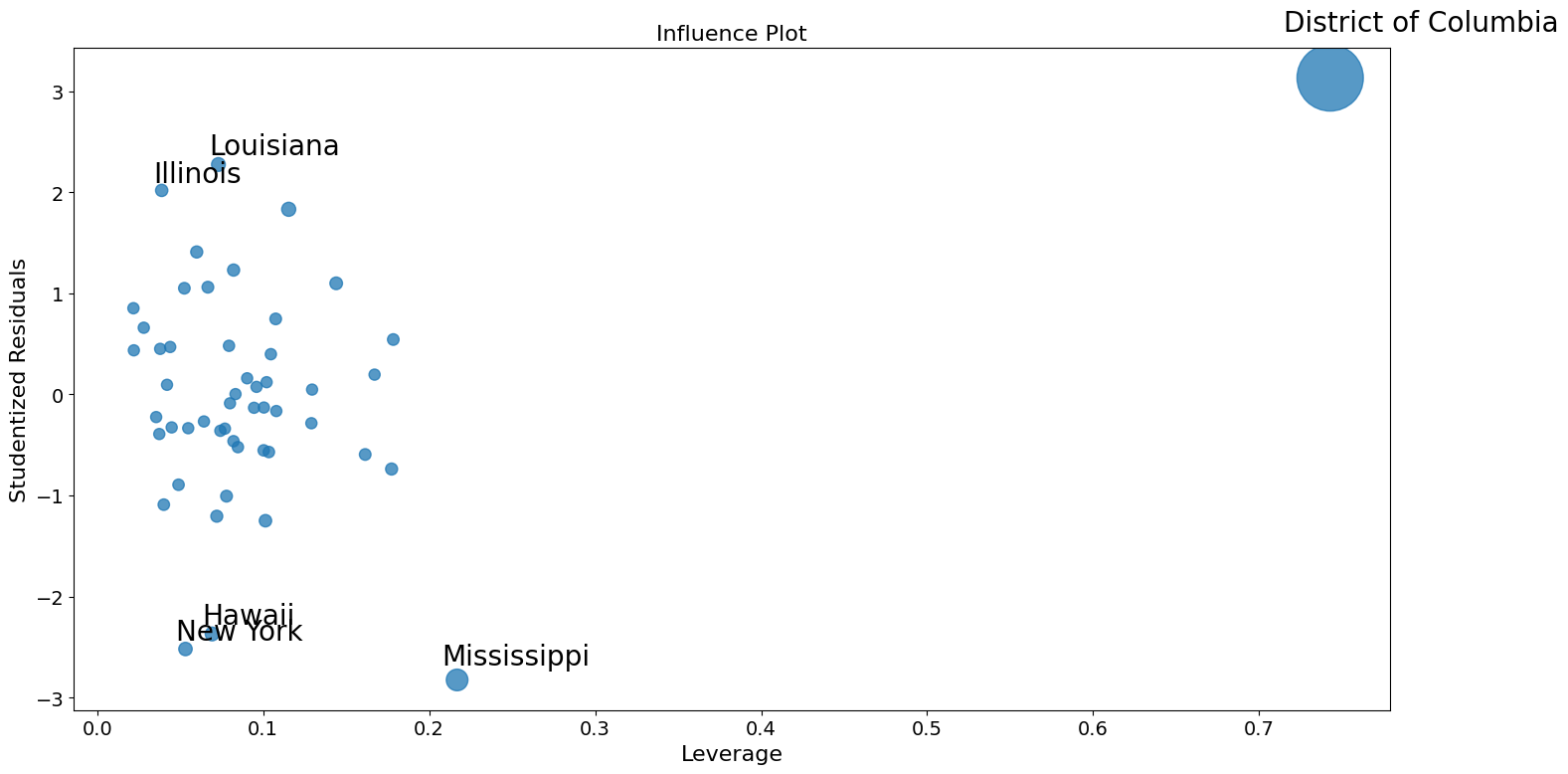
インフルエンスプロット
[22]:
fig = sm.graphics.influence_plot(crime_model)
fig.tight_layout(pad=1.0)
外れ値を補正するためのロバスト回帰の使用
Stata の結果を再現する際のここでの問題の一部は、M推定量がレバレッジポイントを活用するにあたって堅牢ではないことです。MM 推定量は、この例に対してより優れた結果を出すはずです。
[23]:
from statsmodels.formula.api import rlm
[24]:
rob_crime_model = rlm(
    "murder ~ urban + poverty + hs_grad + single",
    data=dta,
    M=sm.robust.norms.TukeyBiweight(3),
).fit(conv="weights")
print(rob_crime_model.summary())
                    Robust linear Model Regression Results
==============================================================================
Dep. Variable:                 murder   No. Observations:                   51
Model:                            RLM   Df Residuals:                       46
Method:                          IRLS   Df Model:                            4
Norm:                   TukeyBiweight
Scale Est.:                       mad
Cov Type:                          H1
Date:                Wed, 28 Aug 2024
Time:                        14:31:13
No. Iterations:                    50
==============================================================================
                 coef    std err          z      P>|z|      [0.025      0.975]
------------------------------------------------------------------------------
Intercept     -4.2986      9.494     -0.453      0.651     -22.907      14.310
urban          0.0029      0.012      0.241      0.809      -0.021       0.027
poverty        0.2753      0.110      2.499      0.012       0.059       0.491
hs_grad       -0.0302      0.092     -0.328      0.743      -0.211       0.150
single         0.2902      0.055      5.253      0.000       0.182       0.398
==============================================================================

If the model instance has been used for another fit with different fit parameters, then the fit options might not be the correct ones anymore .
[25]:
# rob_crime_model = rlm("murder ~ pctmetro + poverty + pcths + single", data=dta, M=sm.robust.norms.TukeyBiweight()).fit(conv="weights")
# print(rob_crime_model.summary())
RLMの一部としての影響診断法はまだ存在しませんが、それを再現することは可能です。(これはissue #888の状況に依存します)
[26]:
weights = rob_crime_model.weights
idx = weights > 0
X = rob_crime_model.model.exog[idx.values]
ww = weights[idx] / weights[idx].mean()
hat_matrix_diag = ww * (X * np.linalg.pinv(X).T).sum(1)
resid = rob_crime_model.resid
resid2 = resid ** 2
resid2 /= resid2.sum()
nobs = int(idx.sum())
hm = hat_matrix_diag.mean()
rm = resid2.mean()
[27]:
from statsmodels.graphics import utils

fig, ax = plt.subplots(figsize=(16, 8))
ax.plot(resid2[idx], hat_matrix_diag, "o")
ax = utils.annotate_axes(
    range(nobs),
    labels=rob_crime_model.model.data.row_labels[idx],
    points=lzip(resid2[idx], hat_matrix_diag),
    offset_points=[(-5, 5)] * nobs,
    size="large",
    ax=ax,
)
ax.set_xlabel("resid2")
ax.set_ylabel("leverage")
ylim = ax.get_ylim()
ax.vlines(rm, *ylim)
xlim = ax.get_xlim()
ax.hlines(hm, *xlim)
ax.margins(0, 0)