ロバスト線形モデル
[1]:
%matplotlib inline
[2]:
import matplotlib.pyplot as plt
import numpy as np
import statsmodels.api as sm
推定
データをロードします:
[3]:
data = sm.datasets.stackloss.load()
data.exog = sm.add_constant(data.exog)
Huberの T ノルム(デフォルトの中央値絶対偏差スケーリング付き)
[4]:
huber_t = sm.RLM(data.endog, data.exog, M=sm.robust.norms.HuberT())
hub_results = huber_t.fit()
print(hub_results.params)
print(hub_results.bse)
print(
    hub_results.summary(
        yname="y", xname=["var_%d" % i for i in range(len(hub_results.params))]
    )
)
const       -41.026498
AIRFLOW       0.829384
WATERTEMP     0.926066
ACIDCONC     -0.127847
dtype: float64
const        9.791899
AIRFLOW      0.111005
WATERTEMP    0.302930
ACIDCONC     0.128650
dtype: float64
                    Robust linear Model Regression Results
==============================================================================
Dep. Variable:                      y   No. Observations:                   21
Model:                            RLM   Df Residuals:                       17
Method:                          IRLS   Df Model:                            3
Norm:                          HuberT
Scale Est.:                       mad
Cov Type:                          H1
Date:                Wed, 28 Aug 2024
Time:                        14:31:34
No. Iterations:                    19
==============================================================================
                 coef    std err          z      P>|z|      [0.025      0.975]
------------------------------------------------------------------------------
var_0        -41.0265      9.792     -4.190      0.000     -60.218     -21.835
var_1          0.8294      0.111      7.472      0.000       0.612       1.047
var_2          0.9261      0.303      3.057      0.002       0.332       1.520
var_3         -0.1278      0.129     -0.994      0.320      -0.380       0.124
==============================================================================

If the model instance has been used for another fit with different fit parameters, then the fit options might not be the correct ones anymore .
Huber の T ノルムと 『H2』 共分散行列
[5]:
hub_results2 = huber_t.fit(cov="H2")
print(hub_results2.params)
print(hub_results2.bse)
const       -41.026498
AIRFLOW       0.829384
WATERTEMP     0.926066
ACIDCONC     -0.127847
dtype: float64
const        9.089504
AIRFLOW      0.119460
WATERTEMP    0.322355
ACIDCONC     0.117963
dtype: float64
Andrewのウェーブノルムと Huber の提案 2 によるスケーリング、および 『H3』 共分散行列
[6]:
andrew_mod = sm.RLM(data.endog, data.exog, M=sm.robust.norms.AndrewWave())
andrew_results = andrew_mod.fit(scale_est=sm.robust.scale.HuberScale(), cov="H3")
print("Parameters: ", andrew_results.params)
Parameters:  const       -40.881796
AIRFLOW       0.792761
WATERTEMP     1.048576
ACIDCONC     -0.133609
dtype: float64
help(sm.RLM.fit) を参照して、さらに多くのオプションを確認してください。また、スケールオプションについては module sm.robust.scale を参照してください。
OLSとRLMの比較
外れ値を含む人工的なデータ:
[7]:
nsample = 50
x1 = np.linspace(0, 20, nsample)
X = np.column_stack((x1, (x1 - 5) ** 2))
X = sm.add_constant(X)
sig = 0.3  # smaller error variance makes OLS<->RLM contrast bigger
beta = [5, 0.5, -0.0]
y_true2 = np.dot(X, beta)
y2 = y_true2 + sig * 1.0 * np.random.normal(size=nsample)
y2[[39, 41, 43, 45, 48]] -= 5  # add some outliers (10% of nsample)
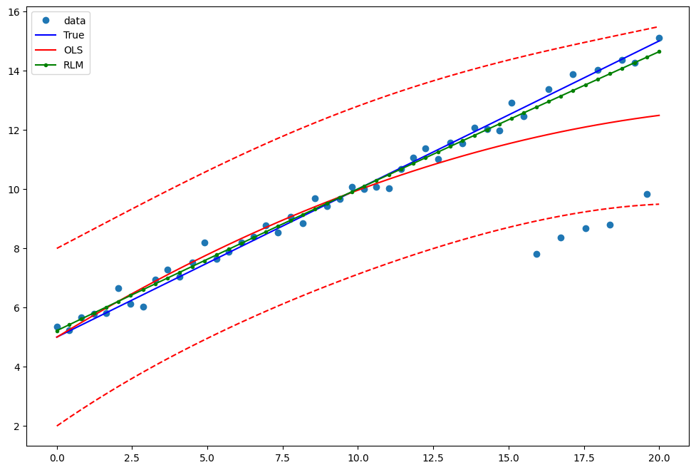
例1: 線形の真実を持つ2次関数
OLS 回帰における 2 次項は、外れ値の影響を捉えることに注意してください。
[8]:
res = sm.OLS(y2, X).fit()
print(res.params)
print(res.bse)
print(res.predict())
[ 5.30093889  0.49657397 -0.01220328]
[0.46069159 0.07112456 0.00629343]
[ 4.99585691  5.24631643  5.49270989  5.73503729  5.97329862  6.20749388
  6.43762308  6.66368621  6.88568327  7.10361427  7.31747921  7.52727808
  7.73301088  7.93467762  8.13227829  8.3258129   8.51528144  8.70068392
  8.88202033  9.05929067  9.23249495  9.40163316  9.56670531  9.72771139
  9.88465141 10.03752536 10.18633324 10.33107506 10.47175081 10.6083605
 10.74090413 10.86938168 10.99379317 11.1141386  11.23041796 11.34263125
 11.45077848 11.55485964 11.65487474 11.75082377 11.84270674 11.93052364
 12.01427448 12.09395924 12.16957795 12.24113059 12.30861716 12.37203767
 12.43139211 12.48668048]
RLM を推定します:
[9]:
resrlm = sm.RLM(y2, X).fit()
print(resrlm.params)
print(resrlm.bse)
[ 5.23600220e+00  4.78479035e-01 -7.45051604e-04]
[0.12236753 0.0188919  0.00167164]
OLS推定値とロバスト推定値を比較するプロットを描きます。
[10]:
fig = plt.figure(figsize=(12, 8))
ax = fig.add_subplot(111)
ax.plot(x1, y2, "o", label="data")
ax.plot(x1, y_true2, "b-", label="True")
pred_ols = res.get_prediction()
iv_l = pred_ols.summary_frame()["obs_ci_lower"]
iv_u = pred_ols.summary_frame()["obs_ci_upper"]

ax.plot(x1, res.fittedvalues, "r-", label="OLS")
ax.plot(x1, iv_u, "r--")
ax.plot(x1, iv_l, "r--")
ax.plot(x1, resrlm.fittedvalues, "g.-", label="RLM")
ax.legend(loc="best")
[10]:
<matplotlib.legend.Legend at 0x1ed79f77640>
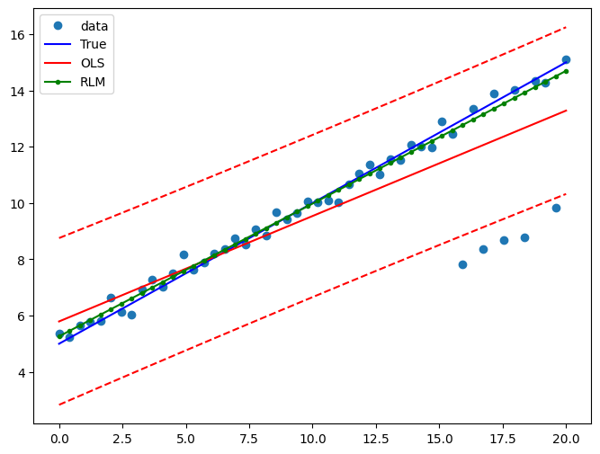
例2: 線形関数と線形真実
線形項と定数項のみを使用して、新しいOLSモデルをフィットさせます。
[11]:
X2 = X[:, [0, 1]]
res2 = sm.OLS(y2, X2).fit()
print(res2.params)
print(res2.bse)
[5.79280577 0.37454118]
[0.39546813 0.03407513]
RLM を推定します:
[12]:
resrlm2 = sm.RLM(y2, X2).fit()
print(resrlm2.params)
print(resrlm2.bse)
[5.26295338 0.47167167]
[0.09662735 0.0083258 ]
OLS推定値とロバスト推定値を比較するプロットを描画します。
[13]:
pred_ols = res2.get_prediction()
iv_l = pred_ols.summary_frame()["obs_ci_lower"]
iv_u = pred_ols.summary_frame()["obs_ci_upper"]

fig, ax = plt.subplots(figsize=(8, 6))
ax.plot(x1, y2, "o", label="data")
ax.plot(x1, y_true2, "b-", label="True")
ax.plot(x1, res2.fittedvalues, "r-", label="OLS")
ax.plot(x1, iv_u, "r--")
ax.plot(x1, iv_l, "r--")
ax.plot(x1, resrlm2.fittedvalues, "g.-", label="RLM")
legend = ax.legend(loc="best")
最終更新日:
2025年01月28日