Statsmodels におけるメタ分析
Statsmodels にはメタ分析のための基本的な方法が含まれています。このノートブックでは現在の使用法を示します。
ステータス: 結果は R の meta および metafor パッケージと照合して確認されています。ただし、API はまだ実験的であり、変更される可能性があります。R の meta および metafor パッケージで利用できる追加の方法のいくつかは、現在サポートされていません。
メタ分析のサポートには 3 つの部分があります:
効果量関数: 現在、次のものが含まれています
effectsize_smdは標準化平均差の効果量とその標準誤差を計算します。effectsize_2proportionsはリスク差、(対数)リスク比、(対数)オッズ比、またはアークサイン平方根変換を使用して、2つの独立した比率を比較するための効果量を計算します。
combine_effectsは、全体の平均または効果の固定効果およびランダム効果の推定値を計算します。返される結果インスタンスには、フォレストプロット関数が含まれています。ランダム効果分散、tau-squared を推定するための補助関数
combine_effects における全体の効果量の推定は、WLS や GLM を使用して var_weights で行うこともできます。
最後に、現在のメタ分析関数には マンテル・ハンゼル(Mantel-Hanszel)法は含まれていません。ただし、固定効果の結果は、以下に示すように StratifiedTable を使用して直接計算することができます。
[1]:
%matplotlib inline
[2]:
import numpy as np
import pandas as pd
from scipy import stats, optimize

from statsmodels.regression.linear_model import WLS
from statsmodels.genmod.generalized_linear_model import GLM

from statsmodels.stats.meta_analysis import (
    effectsize_smd,
    effectsize_2proportions,
    combine_effects,
    _fit_tau_iterative,
    _fit_tau_mm,
    _fit_tau_iter_mm,
)

# increase line length for pandas
pd.set_option("display.width", 100)
例
[3]:
data = [
    ["Carroll", 94, 22, 60, 92, 20, 60],
    ["Grant", 98, 21, 65, 92, 22, 65],
    ["Peck", 98, 28, 40, 88, 26, 40],
    ["Donat", 94, 19, 200, 82, 17, 200],
    ["Stewart", 98, 21, 50, 88, 22, 45],
    ["Young", 96, 21, 85, 92, 22, 85],
]
colnames = ["study", "mean_t", "sd_t", "n_t", "mean_c", "sd_c", "n_c"]
rownames = [i[0] for i in data]
dframe1 = pd.DataFrame(data, columns=colnames)
rownames
[3]:
['Carroll', 'Grant', 'Peck', 'Donat', 'Stewart', 'Young']
[4]:
mean2, sd2, nobs2, mean1, sd1, nobs1 = np.asarray(
    dframe1[["mean_t", "sd_t", "n_t", "mean_c", "sd_c", "n_c"]]
).T
rownames = dframe1["study"]
rownames.tolist()
[4]:
['Carroll', 'Grant', 'Peck', 'Donat', 'Stewart', 'Young']
[5]:
np.array(nobs1 + nobs2)
[5]:
array([120, 130, 80, 400, 95, 170], dtype=int64)
標準化された平均差の効果量を推定する
[6]:
eff, var_eff = effectsize_smd(mean2, sd2, nobs2, mean1, sd1, nobs1)
一段階のカイ二乗検定、DerSimonian-Laird法によるランダム効果分散τの推定
method_re="chi2" または method_re="dl" は、どちらの名前も受け入れられます。[7]:
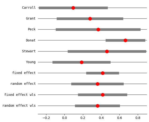
res3 = combine_effects(eff, var_eff, method_re="chi2", use_t=True, row_names=rownames)
# TODO: we still need better information about conf_int of individual samples
# We don't have enough information in the model for individual confidence intervals
# if those are not based on normal distribution.
res3.conf_int_samples(nobs=np.array(nobs1 + nobs2))
print(res3.summary_frame())
                        eff    sd_eff    ci_low    ci_upp      w_fe      w_re
Carroll            0.094524  0.182680 -0.267199  0.456248  0.123885  0.157529
Grant              0.277356  0.176279 -0.071416  0.626129  0.133045  0.162828
Peck               0.366546  0.225573 -0.082446  0.815538  0.081250  0.126223
Donat              0.664385  0.102748  0.462389  0.866381  0.391606  0.232734
Stewart            0.461808  0.208310  0.048203  0.875413  0.095275  0.137949
Young              0.185165  0.153729 -0.118312  0.488641  0.174939  0.182736
fixed effect       0.414961  0.064298  0.249677  0.580245  1.000000       NaN
random effect      0.358486  0.105462  0.087388  0.629583       NaN  1.000000
fixed effect wls   0.414961  0.099237  0.159864  0.670058  1.000000       NaN
random effect wls  0.358486  0.090328  0.126290  0.590682       NaN  1.000000
[8]:
res3.cache_ci
[8]:
{(0.05,
  True): (array([-0.26719942, -0.07141628, -0.08244568,  0.46238908,  0.04820269,
         -0.1183121 ]), array([0.45624817, 0.62612908, 0.81553838, 0.86638112, 0.87541326,
         0.48864139]))}
[9]:
res3.method_re
[9]:
'chi2'
[10]:
fig = res3.plot_forest()
fig.set_figheight(6)
fig.set_figwidth(6)
[11]:
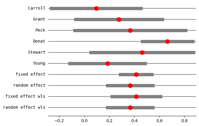
res3 = combine_effects(eff, var_eff, method_re="chi2", use_t=False, row_names=rownames)
# TODO: we still need better information about conf_int of individual samples
# We don't have enough information in the model for individual confidence intervals
# if those are not based on normal distribution.
res3.conf_int_samples(nobs=np.array(nobs1 + nobs2))
print(res3.summary_frame())
                        eff    sd_eff    ci_low    ci_upp      w_fe      w_re
Carroll            0.094524  0.182680 -0.263521  0.452570  0.123885  0.157529
Grant              0.277356  0.176279 -0.068144  0.622857  0.133045  0.162828
Peck               0.366546  0.225573 -0.075569  0.808662  0.081250  0.126223
Donat              0.664385  0.102748  0.463002  0.865768  0.391606  0.232734
Stewart            0.461808  0.208310  0.053527  0.870089  0.095275  0.137949
Young              0.185165  0.153729 -0.116139  0.486468  0.174939  0.182736
fixed effect       0.414961  0.064298  0.288939  0.540984  1.000000       NaN
random effect      0.358486  0.105462  0.151785  0.565187       NaN  1.000000
fixed effect wls   0.414961  0.099237  0.220460  0.609462  1.000000       NaN
random effect wls  0.358486  0.090328  0.181446  0.535526       NaN  1.000000
ランダム効果分散τの反復型 Paule-Mandel 推定の使用
一般に Paule-Mandel 推定と呼ばれる方法は、収束するまで平均と分散の推定を反復する、ランダム効果分散のモーメント推定法です。
[12]:
res4 = combine_effects(
    eff, var_eff, method_re="iterated", use_t=False, row_names=rownames
)
res4_df = res4.summary_frame()
print("method RE:", res4.method_re)
print(res4.summary_frame())
fig = res4.plot_forest()
method RE: iterated
                        eff    sd_eff    ci_low    ci_upp      w_fe      w_re
Carroll            0.094524  0.182680 -0.263521  0.452570  0.123885  0.152619
Grant              0.277356  0.176279 -0.068144  0.622857  0.133045  0.159157
Peck               0.366546  0.225573 -0.075569  0.808662  0.081250  0.116228
Donat              0.664385  0.102748  0.463002  0.865768  0.391606  0.257767
Stewart            0.461808  0.208310  0.053527  0.870089  0.095275  0.129428
Young              0.185165  0.153729 -0.116139  0.486468  0.174939  0.184799
fixed effect       0.414961  0.064298  0.288939  0.540984  1.000000       NaN
random effect      0.366419  0.092390  0.185338  0.547500       NaN  1.000000
fixed effect wls   0.414961  0.099237  0.220460  0.609462  1.000000       NaN
random effect wls  0.366419  0.092390  0.185338  0.547500       NaN  1.000000
[ ]:
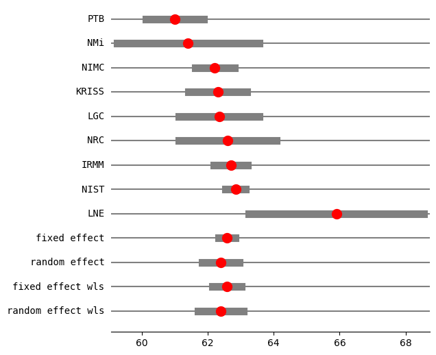
例:Kacker インタラボラトリ平均
この例では、効果量はラボでの測定値の平均です。複数のラボからの推定値を組み合わせて、全体の平均を推定します。
[13]:
eff = np.array([61.00, 61.40, 62.21, 62.30, 62.34, 62.60, 62.70, 62.84, 65.90])
var_eff = np.array(
    [0.2025, 1.2100, 0.0900, 0.2025, 0.3844, 0.5625, 0.0676, 0.0225, 1.8225]
)
rownames = ["PTB", "NMi", "NIMC", "KRISS", "LGC", "NRC", "IRMM", "NIST", "LNE"]
[14]:
res2_DL = combine_effects(eff, var_eff, method_re="dl", use_t=True, row_names=rownames)
print("method RE:", res2_DL.method_re)
print(res2_DL.summary_frame())
fig = res2_DL.plot_forest()
fig.set_figheight(6)
fig.set_figwidth(6)
method RE: dl
                         eff    sd_eff     ci_low     ci_upp      w_fe      w_re
PTB                61.000000  0.450000  60.118016  61.881984  0.057436  0.123113
NMi                61.400000  1.100000  59.244040  63.555960  0.009612  0.040314
NIMC               62.210000  0.300000  61.622011  62.797989  0.129230  0.159749
KRISS              62.300000  0.450000  61.418016  63.181984  0.057436  0.123113
LGC                62.340000  0.620000  61.124822  63.555178  0.030257  0.089810
NRC                62.600000  0.750000  61.130027  64.069973  0.020677  0.071005
IRMM               62.700000  0.260000  62.190409  63.209591  0.172052  0.169810
NIST               62.840000  0.150000  62.546005  63.133995  0.516920  0.194471
LNE                65.900000  1.350000  63.254049  68.545951  0.006382  0.028615
fixed effect       62.583397  0.107846  62.334704  62.832090  1.000000       NaN
random effect      62.390139  0.245750  61.823439  62.956838       NaN  1.000000
fixed effect wls   62.583397  0.189889  62.145512  63.021282  1.000000       NaN
random effect wls  62.390139  0.294776  61.710384  63.069893       NaN  1.000000
C:\Users\user\projects\statsmodels\venv\lib\site-packages\statsmodels\stats\meta_analysis.py:105: UserWarning: `use_t=True` requires `nobs` for each sample or `ci_func`. Using normal distribution for confidence interval of individual samples.
  warnings.warn(msg)
[15]:
res2_PM = combine_effects(eff, var_eff, method_re="pm", use_t=True, row_names=rownames)
print("method RE:", res2_PM.method_re)
print(res2_PM.summary_frame())
fig = res2_PM.plot_forest()
fig.set_figheight(6)
fig.set_figwidth(6)
method RE: pm
                         eff    sd_eff     ci_low     ci_upp      w_fe      w_re
PTB                61.000000  0.450000  60.118016  61.881984  0.057436  0.125857
NMi                61.400000  1.100000  59.244040  63.555960  0.009612  0.059656
NIMC               62.210000  0.300000  61.622011  62.797989  0.129230  0.143658
KRISS              62.300000  0.450000  61.418016  63.181984  0.057436  0.125857
LGC                62.340000  0.620000  61.124822  63.555178  0.030257  0.104850
NRC                62.600000  0.750000  61.130027  64.069973  0.020677  0.090122
IRMM               62.700000  0.260000  62.190409  63.209591  0.172052  0.147821
NIST               62.840000  0.150000  62.546005  63.133995  0.516920  0.156980
LNE                65.900000  1.350000  63.254049  68.545951  0.006382  0.045201
fixed effect       62.583397  0.107846  62.334704  62.832090  1.000000       NaN
random effect      62.407620  0.338030  61.628120  63.187119       NaN  1.000000
fixed effect wls   62.583397  0.189889  62.145512  63.021282  1.000000       NaN
random effect wls  62.407620  0.338030  61.628120  63.187120       NaN  1.000000
C:\Users\user\projects\statsmodels\venv\lib\site-packages\statsmodels\stats\meta_analysis.py:105: UserWarning: `use_t=True` requires `nobs` for each sample or `ci_func`. Using normal distribution for confidence interval of individual samples.
  warnings.warn(msg)

[ ]:
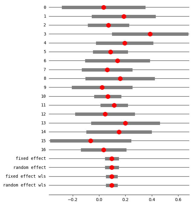
比率のメタ分析
次の例では、ランダム効果の分散τがゼロであると推定されます。その後、データの2つのカウントを変更し、2番目の例ではランダム効果の分散がゼロより大きくなります。
[16]:
import io
[17]:
ss = """\
    study,nei,nci,e1i,c1i,e2i,c2i,e3i,c3i,e4i,c4i
    1,19,22,16.0,20.0,11,12,4.0,8.0,4,3
    2,34,35,22.0,22.0,18,12,15.0,8.0,15,6
    3,72,68,44.0,40.0,21,15,10.0,3.0,3,0
    4,22,20,19.0,12.0,14,5,5.0,4.0,2,3
    5,70,32,62.0,27.0,42,13,26.0,6.0,15,5
    6,183,94,130.0,65.0,80,33,47.0,14.0,30,11
    7,26,50,24.0,30.0,13,18,5.0,10.0,3,9
    8,61,55,51.0,44.0,37,30,19.0,19.0,11,15
    9,36,25,30.0,17.0,23,12,13.0,4.0,10,4
    10,45,35,43.0,35.0,19,14,8.0,4.0,6,0
    11,246,208,169.0,139.0,106,76,67.0,42.0,51,35
    12,386,141,279.0,97.0,170,46,97.0,21.0,73,8
    13,59,32,56.0,30.0,34,17,21.0,9.0,20,7
    14,45,15,42.0,10.0,18,3,9.0,1.0,9,1
    15,14,18,14.0,18.0,13,14,12.0,13.0,9,12
    16,26,19,21.0,15.0,12,10,6.0,4.0,5,1
    17,74,75,,,42,40,,,23,30"""
df3 = pd.read_csv(io.StringIO(ss))
df_12y = df3[["e2i", "nei", "c2i", "nci"]]
# TODO: currently 1 is reference, switch labels
count1, nobs1, count2, nobs2 = df_12y.values.T
dta = df_12y.values.T
[18]:
eff, var_eff = effectsize_2proportions(*dta, statistic="rd")
[19]:
eff, var_eff
[19]:
(array([ 0.03349282,  0.18655462,  0.07107843,  0.38636364,  0.19375   ,
         0.08609464,  0.14      ,  0.06110283,  0.15888889,  0.02222222,
         0.06550969,  0.11417337,  0.04502119,  0.2       ,  0.15079365,
        -0.06477733,  0.03423423]),
 array([0.02409958, 0.01376482, 0.00539777, 0.01989341, 0.01096641,
        0.00376814, 0.01422338, 0.00842011, 0.01639261, 0.01227827,
        0.00211165, 0.00219739, 0.01192067, 0.016     , 0.0143398 ,
        0.02267994, 0.0066352 ]))
[20]:
res5 = combine_effects(
    eff, var_eff, method_re="iterated", use_t=False
)  # , row_names=rownames)
res5_df = res5.summary_frame()
print("method RE:", res5.method_re)
print("RE variance tau2:", res5.tau2)
print(res5.summary_frame())
fig = res5.plot_forest()
fig.set_figheight(8)
fig.set_figwidth(6)
method RE: iterated
RE variance tau2: 0
                        eff    sd_eff    ci_low    ci_upp      w_fe      w_re
0                  0.033493  0.155240 -0.270773  0.337758  0.017454  0.017454
1                  0.186555  0.117324 -0.043395  0.416505  0.030559  0.030559
2                  0.071078  0.073470 -0.072919  0.215076  0.077928  0.077928
3                  0.386364  0.141044  0.109922  0.662805  0.021145  0.021145
4                  0.193750  0.104721 -0.011499  0.398999  0.038357  0.038357
5                  0.086095  0.061385 -0.034218  0.206407  0.111630  0.111630
6                  0.140000  0.119262 -0.093749  0.373749  0.029574  0.029574
7                  0.061103  0.091761 -0.118746  0.240951  0.049956  0.049956
8                  0.158889  0.128034 -0.092052  0.409830  0.025660  0.025660
9                  0.022222  0.110807 -0.194956  0.239401  0.034259  0.034259
10                 0.065510  0.045953 -0.024556  0.155575  0.199199  0.199199
11                 0.114173  0.046876  0.022297  0.206049  0.191426  0.191426
12                 0.045021  0.109182 -0.168971  0.259014  0.035286  0.035286
13                 0.200000  0.126491 -0.047918  0.447918  0.026290  0.026290
14                 0.150794  0.119749 -0.083910  0.385497  0.029334  0.029334
15                -0.064777  0.150599 -0.359945  0.230390  0.018547  0.018547
16                 0.034234  0.081457 -0.125418  0.193887  0.063395  0.063395
fixed effect       0.096212  0.020509  0.056014  0.136410  1.000000       NaN
random effect      0.096212  0.020509  0.056014  0.136410       NaN  1.000000
fixed effect wls   0.096212  0.016521  0.063831  0.128593  1.000000       NaN
random effect wls  0.096212  0.016521  0.063831  0.128593       NaN  1.000000
正のランダム効果分散を持つデータへの変換
[21]:
dta_c = dta.copy()
dta_c.T[0, 0] = 18
dta_c.T[1, 0] = 22
dta_c.T
[21]:
array([[ 18,  19,  12,  22],
       [ 22,  34,  12,  35],
       [ 21,  72,  15,  68],
       [ 14,  22,   5,  20],
       [ 42,  70,  13,  32],
       [ 80, 183,  33,  94],
       [ 13,  26,  18,  50],
       [ 37,  61,  30,  55],
       [ 23,  36,  12,  25],
       [ 19,  45,  14,  35],
       [106, 246,  76, 208],
       [170, 386,  46, 141],
       [ 34,  59,  17,  32],
       [ 18,  45,   3,  15],
       [ 13,  14,  14,  18],
       [ 12,  26,  10,  19],
       [ 42,  74,  40,  75]], dtype=int64)
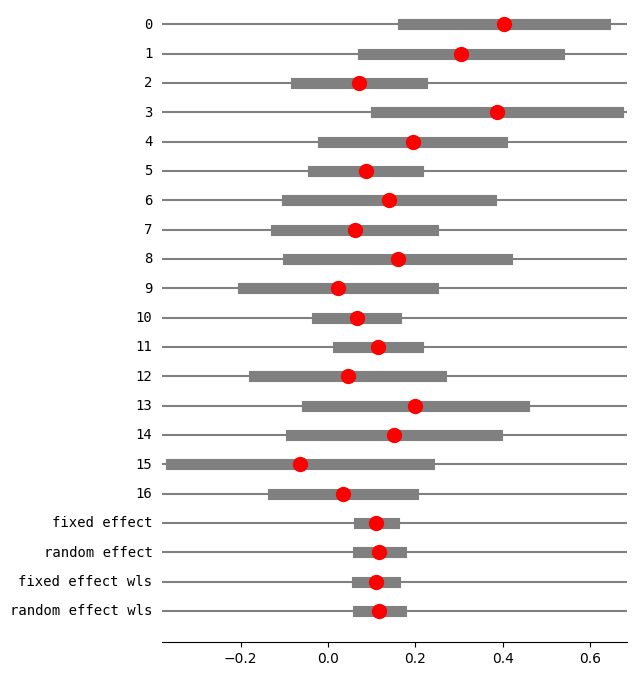
[22]:
eff, var_eff = effectsize_2proportions(*dta_c, statistic="rd")
res5 = combine_effects(
    eff, var_eff, method_re="iterated", use_t=False
)  # , row_names=rownames)
res5_df = res5.summary_frame()
print("method RE:", res5.method_re)
print(res5.summary_frame())
fig = res5.plot_forest()
fig.set_figheight(8)
fig.set_figwidth(6)
method RE: iterated
                        eff    sd_eff    ci_low    ci_upp      w_fe      w_re
0                  0.401914  0.117873  0.170887  0.632940  0.029850  0.038415
1                  0.304202  0.114692  0.079410  0.528993  0.031529  0.040258
2                  0.071078  0.073470 -0.072919  0.215076  0.076834  0.081017
3                  0.386364  0.141044  0.109922  0.662805  0.020848  0.028013
4                  0.193750  0.104721 -0.011499  0.398999  0.037818  0.046915
5                  0.086095  0.061385 -0.034218  0.206407  0.110063  0.102907
6                  0.140000  0.119262 -0.093749  0.373749  0.029159  0.037647
7                  0.061103  0.091761 -0.118746  0.240951  0.049255  0.058097
8                  0.158889  0.128034 -0.092052  0.409830  0.025300  0.033270
9                  0.022222  0.110807 -0.194956  0.239401  0.033778  0.042683
10                 0.065510  0.045953 -0.024556  0.155575  0.196403  0.141871
11                 0.114173  0.046876  0.022297  0.206049  0.188739  0.139144
12                 0.045021  0.109182 -0.168971  0.259014  0.034791  0.043759
13                 0.200000  0.126491 -0.047918  0.447918  0.025921  0.033985
14                 0.150794  0.119749 -0.083910  0.385497  0.028922  0.037383
15                -0.064777  0.150599 -0.359945  0.230390  0.018286  0.024884
16                 0.034234  0.081457 -0.125418  0.193887  0.062505  0.069751
fixed effect       0.110252  0.020365  0.070337  0.150167  1.000000       NaN
random effect      0.117633  0.024913  0.068804  0.166463       NaN  1.000000
fixed effect wls   0.110252  0.022289  0.066567  0.153937  1.000000       NaN
random effect wls  0.117633  0.024913  0.068804  0.166463       NaN  1.000000
[23]:
res5 = combine_effects(eff, var_eff, method_re="chi2", use_t=False)
res5_df = res5.summary_frame()
print("method RE:", res5.method_re)
print(res5.summary_frame())
fig = res5.plot_forest()
fig.set_figheight(8)
fig.set_figwidth(6)
method RE: chi2
                        eff    sd_eff    ci_low    ci_upp      w_fe      w_re
0                  0.401914  0.117873  0.170887  0.632940  0.029850  0.036114
1                  0.304202  0.114692  0.079410  0.528993  0.031529  0.037940
2                  0.071078  0.073470 -0.072919  0.215076  0.076834  0.080779
3                  0.386364  0.141044  0.109922  0.662805  0.020848  0.025973
4                  0.193750  0.104721 -0.011499  0.398999  0.037818  0.044614
5                  0.086095  0.061385 -0.034218  0.206407  0.110063  0.105901
6                  0.140000  0.119262 -0.093749  0.373749  0.029159  0.035356
7                  0.061103  0.091761 -0.118746  0.240951  0.049255  0.056098
8                  0.158889  0.128034 -0.092052  0.409830  0.025300  0.031063
9                  0.022222  0.110807 -0.194956  0.239401  0.033778  0.040357
10                 0.065510  0.045953 -0.024556  0.155575  0.196403  0.154854
11                 0.114173  0.046876  0.022297  0.206049  0.188739  0.151236
12                 0.045021  0.109182 -0.168971  0.259014  0.034791  0.041435
13                 0.200000  0.126491 -0.047918  0.447918  0.025921  0.031761
14                 0.150794  0.119749 -0.083910  0.385497  0.028922  0.035095
15                -0.064777  0.150599 -0.359945  0.230390  0.018286  0.022976
16                 0.034234  0.081457 -0.125418  0.193887  0.062505  0.068449
fixed effect       0.110252  0.020365  0.070337  0.150167  1.000000       NaN
random effect      0.115580  0.023557  0.069410  0.161751       NaN  1.000000
fixed effect wls   0.110252  0.022289  0.066567  0.153937  1.000000       NaN
random effect wls  0.115580  0.024241  0.068068  0.163093       NaN  1.000000

var_weights を使用した固定効果分析の再現
combine_effects は加重平均推定値を計算し、これは var_weights を使用したGLMまたはWLSを使用して再現できます。GLM.fit の scale オプションは、固定効果メタ分析を固定で、またはHKSJ/WLSスケールで再現するために使用できます。[24]:
from statsmodels.genmod.generalized_linear_model import GLM
[25]:
eff, var_eff = effectsize_2proportions(*dta_c, statistic="or")
res = combine_effects(eff, var_eff, method_re="chi2", use_t=False)
res_frame = res.summary_frame()
print(res_frame.iloc[-4:])
                        eff    sd_eff    ci_low    ci_upp  w_fe  w_re
fixed effect       0.428037  0.090287  0.251076  0.604997   1.0   NaN
random effect      0.429520  0.091377  0.250425  0.608615   NaN   1.0
fixed effect wls   0.428037  0.090798  0.250076  0.605997   1.0   NaN
random effect wls  0.429520  0.091595  0.249997  0.609044   NaN   1.0
We need to fix scale=1 in order to replicate standard errors for the usual meta-analysis.
[26]:
weights = 1 / var_eff
mod_glm = GLM(eff, np.ones(len(eff)), var_weights=weights)
res_glm = mod_glm.fit(scale=1.0)
print(res_glm.summary().tables[1])
==============================================================================
                 coef    std err          z      P>|z|      [0.025      0.975]
------------------------------------------------------------------------------
const          0.4280      0.090      4.741      0.000       0.251       0.605
==============================================================================
[27]:
# check results
res_glm.scale, res_glm.conf_int() - res_frame.loc[
    "fixed effect", ["ci_low", "ci_upp"]
].values
[27]:
(array(1.), array([[-5.55111512e-17, 0.00000000e+00]]))
メタ分析でHKSJ分散調整を使用することは、ピアソンのカイ二乗を使用してスケールを推定することと同等であり、これはガウス分布ファミリーのデフォルトでもあります。
[28]:
res_glm = mod_glm.fit(scale="x2")
print(res_glm.summary().tables[1])
==============================================================================
                 coef    std err          z      P>|z|      [0.025      0.975]
------------------------------------------------------------------------------
const          0.4280      0.091      4.714      0.000       0.250       0.606
==============================================================================
[29]:
# check results
res_glm.scale, res_glm.conf_int() - res_frame.loc[
    "fixed effect", ["ci_low", "ci_upp"]
].values
[29]:
(1.0113358914264383, array([[-0.00100017, 0.00100017]]))
マンテル・ハンゼルオッズ比の使用(分割表を用いて)
マンテル・ハンゼル法を使用した対数オッズ比の固定効果は、StratifiedTableを使用して直接計算することができます。
StratifiedTableと共に使用するために、2 x 2 x k の分割表を作成する必要があります。
[30]:
t, nt, c, nc = dta_c
counts = np.column_stack([t, nt - t, c, nc - c])
ctables = counts.T.reshape(2, 2, -1)
ctables[:, :, 0]
[30]:
array([[18,  1],
       [12, 10]], dtype=int64)
[31]:
counts[0]
[31]:
array([18, 1, 12, 10], dtype=int64)
[32]:
dta_c.T[0]
[32]:
array([18, 19, 12, 22], dtype=int64)
[33]:
import statsmodels.stats.api as smstats
[34]:
st = smstats.StratifiedTable(ctables.astype(np.float64))
プールされたログオッズ比と標準誤差をRのメタパッケージと比較する
[35]:
st.logodds_pooled, st.logodds_pooled - 0.4428186730553189 # R meta
[35]:
(0.4428186730553187, -2.220446049250313e-16)
[36]:
st.logodds_pooled_se, st.logodds_pooled_se - 0.08928560091027186 # R meta
[36]:
(0.08928560091027186, 0.0)
[37]:
st.logodds_pooled_confint()
[37]:
(0.2678221109331691, 0.6178152351774683)
[38]:
print(st.test_equal_odds())
pvalue      0.34496419319878713
statistic   17.64707987033203
[39]:
print(st.test_null_odds())
pvalue      6.615053645964153e-07
statistic   24.724136624311814
層別クロス集計表への変換を確認する
各テーブルの行の合計は、処置群とコントロール群の実験における標本サイズです。
[40]:
ctables.sum(1)
[40]:
array([[ 19,  34,  72,  22,  70, 183,  26,  61,  36,  45, 246, 386,  59,
         45,  14,  26,  74],
       [ 22,  35,  68,  20,  32,  94,  50,  55,  25,  35, 208, 141,  32,
         15,  18,  19,  75]], dtype=int64)
[41]:
nt, nc
[41]:
(array([ 19,  34,  72,  22,  70, 183,  26,  61,  36,  45, 246, 386,  59,
         45,  14,  26,  74], dtype=int64),
 array([ 22,  35,  68,  20,  32,  94,  50,  55,  25,  35, 208, 141,  32,
         15,  18,  19,  75], dtype=int64))
Rメタパッケージの結果
> res_mb_hk = metabin(e2i, nei, c2i, nci, data=dat2, sm="OR", Q.Cochrane=FALSE, method="MH", method.tau="DL", hakn=FALSE, backtransf=FALSE)
> res_mb_hk
     logOR            95%-CI %W(fixed) %W(random)
1   2.7081 [ 0.5265; 4.8896]       0.3        0.7
2   1.2567 [ 0.2658; 2.2476]       2.1        3.2
3   0.3749 [-0.3911; 1.1410]       5.4        5.4
4   1.6582 [ 0.3245; 2.9920]       0.9        1.8
5   0.7850 [-0.0673; 1.6372]       3.5        4.4
6   0.3617 [-0.1528; 0.8762]      12.1       11.8
7   0.5754 [-0.3861; 1.5368]       3.0        3.4
8   0.2505 [-0.4881; 0.9892]       6.1        5.8
9   0.6506 [-0.3877; 1.6889]       2.5        3.0
10  0.0918 [-0.8067; 0.9903]       4.5        3.9
11  0.2739 [-0.1047; 0.6525]      23.1       21.4
12  0.4858 [ 0.0804; 0.8911]      18.6       18.8
13  0.1823 [-0.6830; 1.0476]       4.6        4.2
14  0.9808 [-0.4178; 2.3795]       1.3        1.6
15  1.3122 [-1.0055; 3.6299]       0.4        0.6
16 -0.2595 [-1.4450; 0.9260]       3.1        2.3
17  0.1384 [-0.5076; 0.7844]       8.5        7.6

Number of studies combined: k = 17

                      logOR           95%-CI    z  p-value
Fixed effect model   0.4428 [0.2678; 0.6178] 4.96 < 0.0001
Random effects model 0.4295 [0.2504; 0.6086] 4.70 < 0.0001

Quantifying heterogeneity:
 tau^2 = 0.0017 [0.0000; 0.4589]; tau = 0.0410 [0.0000; 0.6774];
 I^2 = 1.1% [0.0%; 51.6%]; H = 1.01 [1.00; 1.44]

Test of heterogeneity:
     Q d.f. p-value
 16.18   16  0.4404

Details on meta-analytical method:
- Mantel-Haenszel method
- DerSimonian-Laird estimator for tau^2
- Jackson method for confidence interval of tau^2 and tau

> res_mb_hk$TE.fixed
[1] 0.4428186730553189
> res_mb_hk$seTE.fixed
[1] 0.08928560091027186
> c(res_mb_hk$lower.fixed, res_mb_hk$upper.fixed)
[1] 0.2678221109331694 0.6178152351774684
[42]:
print(st.summary())
                   Estimate   LCB    UCB
-----------------------------------------
Pooled odds           1.557   1.307 1.855
Pooled log odds       0.443   0.268 0.618
Pooled risk ratio     1.270

                 Statistic P-value
-----------------------------------
Test of OR=1        24.724   0.000
Test constant OR    17.647   0.345

-----------------------
Number of tables   17
Min n              32
Max n             527
Avg n             139
Total n          2362
-----------------------