予測(標本外)
[1]:
%matplotlib inline
[2]:
import numpy as np
import matplotlib.pyplot as plt

import statsmodels.api as sm

plt.rc("figure", figsize=(16, 8))
plt.rc("font", size=14)
人工的データ
[3]:
nsample = 50
sig = 0.25
x1 = np.linspace(0, 20, nsample)
X = np.column_stack((x1, np.sin(x1), (x1 - 5) ** 2))
X = sm.add_constant(X)
beta = [5.0, 0.5, 0.5, -0.02]
y_true = np.dot(X, beta)
y = y_true + sig * np.random.normal(size=nsample)
推定
[4]:
olsmod = sm.OLS(y, X)
olsres = olsmod.fit()
print(olsres.summary())
                            OLS Regression Results
==============================================================================
Dep. Variable:                      y   R-squared:                       0.987
Model:                            OLS   Adj. R-squared:                  0.986
Method:                 Least Squares   F-statistic:                     1178.
Date:                Wed, 28 Aug 2024   Prob (F-statistic):           1.76e-43
Time:                        14:20:45   Log-Likelihood:                 6.2799
No. Observations:                  50   AIC:                            -4.560
Df Residuals:                      46   BIC:                             3.088
Df Model:                           3
Covariance Type:            nonrobust
==============================================================================
                 coef    std err          t      P>|t|      [0.025      0.975]
------------------------------------------------------------------------------
const          5.0108      0.076     66.074      0.000       4.858       5.163
x1             0.4977      0.012     42.556      0.000       0.474       0.521
x2             0.4630      0.046     10.069      0.000       0.370       0.556
x3            -0.0191      0.001    -18.648      0.000      -0.021      -0.017
==============================================================================
Omnibus:                        2.015   Durbin-Watson:                   2.109
Prob(Omnibus):                  0.365   Jarque-Bera (JB):                1.274
Skew:                          -0.368   Prob(JB):                        0.529
Kurtosis:                       3.264   Cond. No.                         221.
==============================================================================

Notes:
[1] Standard Errors assume that the covariance matrix of the errors is correctly specified.
標本内予測
[5]:
ypred = olsres.predict(X)
print(ypred)
[ 4.5320388   4.99392652  5.41924213  5.78275451  6.06833833  6.27162335
  6.40071252  6.47485062  6.52126242  6.57067974  6.65229229  6.78895187
  6.9934179   7.26626108  7.59576963  7.95987349  8.32977037  8.6746579
  8.96679435  9.18605655  9.32324603  9.38160033  9.37626107  9.33178623
  9.27811535  9.24565053  9.26026146  9.33903511  9.48746838  9.69856498
  9.95398489 10.2270576  10.48716397 10.70476688 10.85626409 10.92786603
 10.9178614  10.83689829 10.70623476 10.5542462  10.41176334 10.30700681
 10.26095062 10.28387615 10.37368299 10.51623397 10.68767793 10.85836834
 10.99773417 11.07930261]
新しい説明変数 Xnew を作成し、予測してプロットする
[6]:
x1n = np.linspace(20.5, 25, 10)
Xnew = np.column_stack((x1n, np.sin(x1n), (x1n - 5) ** 2))
Xnew = sm.add_constant(Xnew)
ynewpred = olsres.predict(Xnew)  # predict out of sample
print(ynewpred)
[11.07496821 10.94806855 10.71675933 10.42241509 10.11949925  9.86222964
  9.691304    9.62393579  9.64963977  9.73279908]
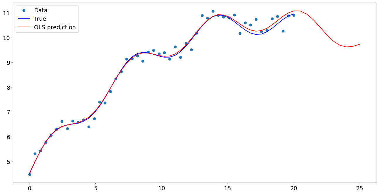
プロット比較
[7]:
import matplotlib.pyplot as plt

fig, ax = plt.subplots()
ax.plot(x1, y, "o", label="Data")
ax.plot(x1, y_true, "b-", label="True")
ax.plot(np.hstack((x1, x1n)), np.hstack((ypred, ynewpred)), "r", label="OLS prediction")
ax.legend(loc="best")
[7]:
<matplotlib.legend.Legend at 0x11db709d270>
数式を使った予測
公式を使うことで、推定と予測の両方がずっと簡単になります。
[8]:
from statsmodels.formula.api import ols

data = {"x1": x1, "y": y}

res = ols("y ~ x1 + np.sin(x1) + I((x1-5)**2)", data=data).fit()
I を使用して、恒等変換の使用を示します。つまり、**2 を使って展開の魔法を適用したくないという意味です。
[9]:
res.params
[9]:
Intercept           5.010783
x1                  0.497728
np.sin(x1)          0.462964
I((x1 - 5) ** 2)   -0.019150
dtype: float64
これで、1つの変数を渡すだけで、変換された右辺の変数が自動的に取得されます。
[10]:
res.predict(exog=dict(x1=x1n))
[10]:
0    11.074968
1    10.948069
2    10.716759
3    10.422415
4    10.119499
5     9.862230
6     9.691304
7     9.623936
8     9.649640
9     9.732799
dtype: float64
最終更新日:
2025年01月28日