statsmodels における予測
このノートブックでは、statsmodels を使用した時系列モデルによる予測について説明します。
注: このノートブックは、状態空間モデルクラスにのみ適用されます。これらのクラスは以下の通りです:
sm.tsa.SARIMAXsm.tsa.UnobservedComponentssm.tsa.VARMAXsm.tsa.DynamicFactor
[1]:
%matplotlib inline

import numpy as np
import pandas as pd
import statsmodels.api as sm
import matplotlib.pyplot as plt

macrodata = sm.datasets.macrodata.load_pandas().data
macrodata.index = pd.period_range('1959Q1', '2009Q3', freq='Q')
基本的な例
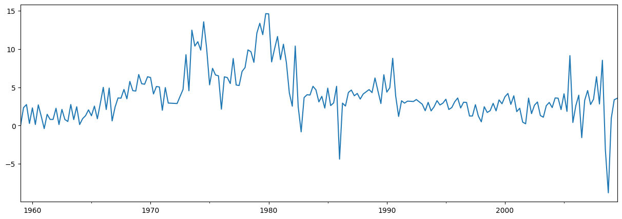
シンプルな例として、AR(1)モデルを使用してインフレを予測します。予測を行う前に、まずはその時系列を見てみましょう:
[2]:
endog = macrodata['infl']
endog.plot(figsize=(15, 5))
[2]:
<Axes: >
モデルの構築と推定
次のステップは、予測に使用する計量経済学モデルを定式化することです。この場合、SARIMAX クラスを使用してAR(1)モデルを利用します。
モデルを構築した後、次はそのパラメータを推定する必要があります。これには、fit メソッドを使用します。summary メソッドは、結果を示すいくつかの便利なテーブルを生成します。
[3]:
# Construct the model
mod = sm.tsa.SARIMAX(endog, order=(1, 0, 0), trend='c')
# Estimate the parameters
res = mod.fit()

print(res.summary())
                               SARIMAX Results
==============================================================================
Dep. Variable:                   infl   No. Observations:                  203
Model:               SARIMAX(1, 0, 0)   Log Likelihood                -472.714
Date:                Thu, 28 Nov 2024   AIC                            951.427
Time:                        23:11:42   BIC                            961.367
Sample:                    03-31-1959   HQIC                           955.449
                         - 09-30-2009
Covariance Type:                  opg
==============================================================================
                 coef    std err          z      P>|z|      [0.025      0.975]
------------------------------------------------------------------------------
intercept      1.3962      0.254      5.488      0.000       0.898       1.895
ar.L1          0.6441      0.039     16.482      0.000       0.568       0.721
sigma2         6.1519      0.397     15.487      0.000       5.373       6.930
===================================================================================
Ljung-Box (L1) (Q):                   8.43   Jarque-Bera (JB):                68.45
Prob(Q):                              0.00   Prob(JB):                         0.00
Heteroskedasticity (H):               1.47   Skew:                            -0.22
Prob(H) (two-sided):                  0.12   Kurtosis:                         5.81
===================================================================================

Warnings:
[1] Covariance matrix calculated using the outer product of gradients (complex-step).
予測
標本外の予測は、結果オブジェクトの forecast または get_forecast メソッドを使用して生成されます。
forecast メソッドは、点予測のみを提供します。
[4]:
# The default is to get a one-step-ahead forecast:
print(res.forecast())
2009Q4    3.68921
Freq: Q-DEC, dtype: float64
get_forecast メソッドはより一般的で、信頼区間の構築も可能です。
[5]:
# Here we construct a more complete results object.
fcast_res1 = res.get_forecast()

# Most results are collected in the `summary_frame` attribute.
# Here we specify that we want a confidence level of 90%
print(fcast_res1.summary_frame(alpha=0.10))
infl       mean   mean_se  mean_ci_lower  mean_ci_upper
2009Q4  3.68921  2.480302      -0.390523       7.768943
デフォルトの信頼水準は95%ですが、これは alpha パラメータを設定することで調整できます。信頼水準は \((1 - \alpha) \times 100\%\) と定義されます。上記の例では、信頼水準を90%に指定するために alpha=0.10 を使用しました。
予測ステップの数の指定
forecast 関数と get_forecast 関数の両方は、希望する予測ステップ数を示す単一の引数を受け入れます。この引数のオプションの1つは、予測したいステップ数を表す整数を提供することです。
[6]:
print(res.forecast(steps=2))
2009Q4    3.689210
2010Q1    3.772434
Freq: Q-DEC, Name: predicted_mean, dtype: float64
[7]:
fcast_res2 = res.get_forecast(steps=2)
# Note: since we did not specify the alpha parameter, the
# confidence level is at the default, 95%
print(fcast_res2.summary_frame())
infl        mean   mean_se  mean_ci_lower  mean_ci_upper
2009Q4  3.689210  2.480302      -1.172092       8.550512
2010Q1  3.772434  2.950274      -2.009996       9.554865
ただし、データに定義された頻度を持つPandasのインデックスが含まれている場合(インデックスに関する詳細は最後のセクションを参照)、予測を生成したい日付を指定することもできます。
[8]:
print(res.forecast('2010Q2'))
2009Q4    3.689210
2010Q1    3.772434
2010Q2    3.826039
Freq: Q-DEC, Name: predicted_mean, dtype: float64
[9]:
fcast_res3 = res.get_forecast('2010Q2')
print(fcast_res3.summary_frame())
infl        mean   mean_se  mean_ci_lower  mean_ci_upper
2009Q4  3.689210  2.480302      -1.172092       8.550512
2010Q1  3.772434  2.950274      -2.009996       9.554865
2010Q2  3.826039  3.124571      -2.298008       9.950087
データ、予測、信頼区間のプロット
データ、予測、および信頼区間をプロットすることはよく役立ちます。これを行う方法はいくつかありますが、以下はその一例です。
[10]:
fig, ax = plt.subplots(figsize=(15, 5))

# Plot the data (here we are subsetting it to get a better look at the forecasts)
endog.loc['1999':].plot(ax=ax)

# Construct the forecasts
fcast = res.get_forecast('2011Q4').summary_frame()
fcast['mean'].plot(ax=ax, style='k--')
ax.fill_between(fcast.index, fcast['mean_ci_lower'], fcast['mean_ci_upper'], color='k', alpha=0.1);
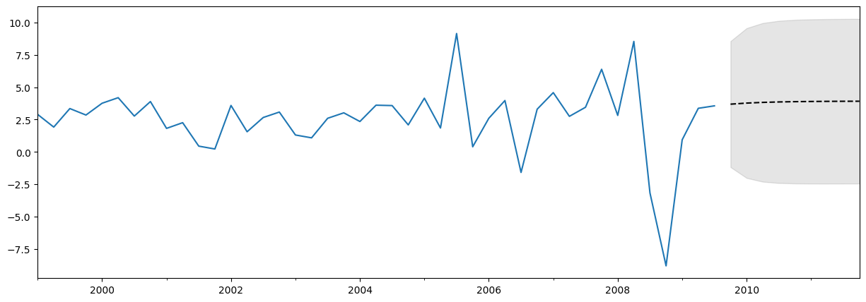
予測結果に関する注意
上記の予測はほとんど直線のように見えるかもしれませんが、これは非常にシンプルな単変量予測モデルだからです。それでも、これらのシンプルな予測モデルが非常に競争力を持つことがあることを忘れないでください。
予測 vs 予測値の予測
結果オブジェクトには、標本内の適合値と標本外の予測の両方に対応する2つのメソッドが含まれています。それらは predict と get_prediction です。predict メソッドはポイント予測のみを返します(forecast と似ています)が、get_prediction メソッドは追加の結果も返します(get_forecast と似ています)。
一般的に、標本外の予測に関心がある場合は、forecast と get_forecast メソッドを使用する方が簡単です。
クロスバリデーション
注: このセクションで使用されているいくつかの関数は、statsmodels v0.11.0で初めて導入されました。
一般的な使用例として、次のプロセスを使用して、予測手法のクロスバリデーションを行うことがあります:
訓練サンプルでモデルパラメータをフィットさせる
サンプルの最後からhステップ先の予測を生成する
テストデータセットと予測を比較し、誤差率を計算する
サンプルを拡張して次の観測値を含め、繰り返す
経済学者はこれを擬似的なサンプル外予測評価演習、または時系列クロスバリデーションと呼ぶことがあります。
例題
上記のインフレデータセットを使用して、このような非常にシンプルな演習を行います。完全なデータセットには203の観測値が含まれており、説明の目的で最初の80%をトレーニングサンプルとして使用し、1ステップ先の予測のみを考慮します。
上記の手順の1回の反復は、次のようになります:
[11]:
# Step 1: fit model parameters w/ training sample
training_obs = int(len(endog) * 0.8)

training_endog = endog[:training_obs]
training_mod = sm.tsa.SARIMAX(
    training_endog, order=(1, 0, 0), trend='c')
training_res = training_mod.fit()

# Print the estimated parameters
print(training_res.params)
intercept    1.162076
ar.L1        0.724242
sigma2       5.051600
dtype: float64
[12]:
# Step 2: produce one-step-ahead forecasts
fcast = training_res.forecast()

# Step 3: compute root mean square forecasting error
true = endog.reindex(fcast.index)
error = true - fcast

# Print out the results
print(pd.concat([true.rename('true'),
                 fcast.rename('forecast'),
                 error.rename('error')], axis=1))
        true  forecast    error
1999Q3  3.35   2.55262  0.79738
もう一つの観測値を追加するには、append または extend メソッドを使用できます。どちらのメソッドでも同じ予測を得ることができますが、利用可能な他の結果が異なります:
appendはより完全な方法です。すべての訓練データに対する結果を常に保存し、新しい観測値が得られた場合にモデルのパラメータを再調整することも可能です(デフォルトではパラメータは再調整しません)。extendはより高速な方法で、訓練標本が非常に大きい場合に役立ちます。新しい観測値に対する結果のみを保存し、モデルのパラメータの再調整は行いません(つまり、前回の標本で推定されたパラメータを使用する必要があります)。
訓練標本が比較的小さい(例えば、数千件未満の観測値)場合や、最良の予測値を計算したい場合は、append メソッドを使用すべきです。しかし、この方法が不可能な場合(例えば、訓練標本が非常に大きい場合)や、若干最適でない予測でも問題ない場合(パラメータ推定が少し古くなるため)、extend メソッドを検討することができます。
2回目の反復では、append メソッドを使用し、パラメータを再フィッティングします。次のように進めます(再度注意ですが、append のデフォルトではパラメータの再フィッティングは行われませんが、refit=True 引数を使用してそれを上書きしています):
[13]:
# Step 1: append a new observation to the sample and refit the parameters
append_res = training_res.append(endog[training_obs:training_obs + 1], refit=True)

# Print the re-estimated parameters
print(append_res.params)
intercept    1.171544
ar.L1        0.723152
sigma2       5.024580
dtype: float64
これらの推定されたパラメータは、元々推定したものとはわずかに異なることに注意してください。新しい結果オブジェクト append_res を使用すると、前回の呼び出しよりも1つ多い観測値から予測を計算することができます。
[14]:
# Step 2: produce one-step-ahead forecasts
fcast = append_res.forecast()

# Step 3: compute root mean square forecasting error
true = endog.reindex(fcast.index)
error = true - fcast

# Print out the results
print(pd.concat([true.rename('true'),
                 fcast.rename('forecast'),
                 error.rename('error')], axis=1))
        true  forecast     error
1999Q4  2.85  3.594102 -0.744102
まとめると、次のように再帰的な予測評価演習を行うことができます:
[15]:
# Setup forecasts
nforecasts = 3
forecasts = {}

# Get the number of initial training observations
nobs = len(endog)
n_init_training = int(nobs * 0.8)

# Create model for initial training sample, fit parameters
init_training_endog = endog.iloc[:n_init_training]
mod = sm.tsa.SARIMAX(training_endog, order=(1, 0, 0), trend='c')
res = mod.fit()

# Save initial forecast
forecasts[training_endog.index[-1]] = res.forecast(steps=nforecasts)

# Step through the rest of the sample
for t in range(n_init_training, nobs):
    # Update the results by appending the next observation
    updated_endog = endog.iloc[t:t+1]
    res = res.append(updated_endog, refit=False)

    # Save the new set of forecasts
    forecasts[updated_endog.index[0]] = res.forecast(steps=nforecasts)

# Combine all forecasts into a dataframe
forecasts = pd.concat(forecasts, axis=1)

print(forecasts.iloc[:5, :5])
          1999Q2    1999Q3    1999Q4    2000Q1    2000Q2
1999Q3  2.552620       NaN       NaN       NaN       NaN
1999Q4  3.010790  3.588286       NaN       NaN       NaN
2000Q1  3.342616  3.760863  3.226165       NaN       NaN
2000Q2       NaN  3.885850  3.498599  3.885225       NaN
2000Q3       NaN       NaN  3.695908  3.975918  4.196649
現在、1999年Q2から2009年Q3までの各時点で作成された3つの予測セットがあります。予測誤差は、各予測からその時点でのendogの実際の値を引くことによって構築できます。
[16]:
# Construct the forecast errors
forecast_errors = forecasts.apply(lambda column: endog - column).reindex(forecasts.index)

print(forecast_errors.iloc[:5, :5])
          1999Q2    1999Q3    1999Q4    2000Q1    2000Q2
1999Q3  0.797380       NaN       NaN       NaN       NaN
1999Q4 -0.160790 -0.738286       NaN       NaN       NaN
2000Q1  0.417384 -0.000863  0.533835       NaN       NaN
2000Q2       NaN  0.304150  0.691401  0.304775       NaN
2000Q3       NaN       NaN -0.925908 -1.205918 -1.426649
予測の評価を行うために、通常は平方平均二乗誤差(RMSE)のような要約値を確認したいと考えます。ここでは、予測誤差をまず水平線でインデックス付けして平坦化し、その後、各水平線に対して平方平均二乗誤差を計算することで、これを行うことができます。
[17]:
# Reindex the forecasts by horizon rather than by date
def flatten(column):
    return column.dropna().reset_index(drop=True)

flattened = forecast_errors.apply(flatten)
flattened.index = (flattened.index + 1).rename('horizon')

print(flattened.iloc[:3, :5])
           1999Q2    1999Q3    1999Q4    2000Q1    2000Q2
horizon
1        0.797380 -0.738286  0.533835  0.304775 -1.426649
2       -0.160790 -0.000863  0.691401 -1.205918 -0.311464
3        0.417384  0.304150 -0.925908 -0.151602 -2.384952
[18]:
# Compute the root mean square error
rmse = (flattened**2).mean(axis=1)**0.5

print(rmse)
horizon
1    3.292700
2    3.421808
3    3.280012
dtype: float64
extend を使用する場合
extend メソッドを使用した場合でも、同様の予測が得られることを確認できますが、refit=True 引数を使って append を使用した場合と正確に同じ結果にはなりません。これは、extend が新しい観測値を考慮してパラメータを再推定しないためです。
[19]:
# Setup forecasts
nforecasts = 3
forecasts = {}

# Get the number of initial training observations
nobs = len(endog)
n_init_training = int(nobs * 0.8)

# Create model for initial training sample, fit parameters
init_training_endog = endog.iloc[:n_init_training]
mod = sm.tsa.SARIMAX(training_endog, order=(1, 0, 0), trend='c')
res = mod.fit()

# Save initial forecast
forecasts[training_endog.index[-1]] = res.forecast(steps=nforecasts)

# Step through the rest of the sample
for t in range(n_init_training, nobs):
    # Update the results by appending the next observation
    updated_endog = endog.iloc[t:t+1]
    res = res.extend(updated_endog)

    # Save the new set of forecasts
    forecasts[updated_endog.index[0]] = res.forecast(steps=nforecasts)

# Combine all forecasts into a dataframe
forecasts = pd.concat(forecasts, axis=1)

print(forecasts.iloc[:5, :5])
          1999Q2    1999Q3    1999Q4    2000Q1    2000Q2
1999Q3  2.552620       NaN       NaN       NaN       NaN
1999Q4  3.010790  3.588286       NaN       NaN       NaN
2000Q1  3.342616  3.760863  3.226165       NaN       NaN
2000Q2       NaN  3.885850  3.498599  3.885225       NaN
2000Q3       NaN       NaN  3.695908  3.975918  4.196649
[20]:
# Construct the forecast errors
forecast_errors = forecasts.apply(lambda column: endog - column).reindex(forecasts.index)

print(forecast_errors.iloc[:5, :5])
          1999Q2    1999Q3    1999Q4    2000Q1    2000Q2
1999Q3  0.797380       NaN       NaN       NaN       NaN
1999Q4 -0.160790 -0.738286       NaN       NaN       NaN
2000Q1  0.417384 -0.000863  0.533835       NaN       NaN
2000Q2       NaN  0.304150  0.691401  0.304775       NaN
2000Q3       NaN       NaN -0.925908 -1.205918 -1.426649
[21]:
# Reindex the forecasts by horizon rather than by date
def flatten(column):
    return column.dropna().reset_index(drop=True)

flattened = forecast_errors.apply(flatten)
flattened.index = (flattened.index + 1).rename('horizon')

print(flattened.iloc[:3, :5])
           1999Q2    1999Q3    1999Q4    2000Q1    2000Q2
horizon
1        0.797380 -0.738286  0.533835  0.304775 -1.426649
2       -0.160790 -0.000863  0.691401 -1.205918 -0.311464
3        0.417384  0.304150 -0.925908 -0.151602 -2.384952
[22]:
# Compute the root mean square error
rmse = (flattened**2).mean(axis=1)**0.5

print(rmse)
horizon
1    3.292700
2    3.421808
3    3.280012
dtype: float64
パラメータを再推定しないことで、予測は若干悪化します(各予測期間において平均二乗誤差が高くなります)。しかし、プロセスは速く、200のデータポイントでも高速です。上記のセルで %%timeit マジックコマンドを使用した結果、extend を使用した場合の実行時間は570ms、refit=True で append を使用した場合は1.7秒でした(なお、extend を使用する方が、refit=False で append を使用するよりも速いことも確認されました)。
インデックス
このノートブック全体で、関連する頻度を持つPandasの日付インデックスを使用してきました。ご覧のように、このインデックスは、1959年第1四半期から2009年第3四半期までの四半期ごとのデータを示しています。
[23]:
print(endog.index)
PeriodIndex(['1959Q1', '1959Q2', '1959Q3', '1959Q4', '1960Q1', '1960Q2',
             '1960Q3', '1960Q4', '1961Q1', '1961Q2',
             ...
             '2007Q2', '2007Q3', '2007Q4', '2008Q1', '2008Q2', '2008Q3',
             '2008Q4', '2009Q1', '2009Q2', '2009Q3'],
            dtype='period[Q-DEC]', length=203)
ほとんどの場合、データに定義された頻度(四半期ごと、月次など)の関連する日付/時刻インデックスがある場合、データが適切なインデックスを持つPandasシリーズであることを確認するのが最適です。以下はその例として3つのケースです:
[24]:
# Annual frequency, using a PeriodIndex
index = pd.period_range(start='2000', periods=4, freq='A')
endog1 = pd.Series([1, 2, 3, 4], index=index)
print(endog1.index)
PeriodIndex(['2000', '2001', '2002', '2003'], dtype='period[Y-DEC]')
C:\Users\user\AppData\Local\Temp\ipykernel_14404\63920926.py:2: FutureWarning: 'A' is deprecated and will be removed in a future version, please use 'Y' instead.
  index = pd.period_range(start='2000', periods=4, freq='A')
[25]:
# Quarterly frequency, using a DatetimeIndex
index = pd.date_range(start='2000', periods=4, freq='QS')
endog2 = pd.Series([1, 2, 3, 4], index=index)
print(endog2.index)
DatetimeIndex(['2000-01-01', '2000-04-01', '2000-07-01', '2000-10-01'], dtype='datetime64[ns]', freq='QS-JAN')
[26]:
# Monthly frequency, using a DatetimeIndex
index = pd.date_range(start='2000', periods=4, freq='M')
endog3 = pd.Series([1, 2, 3, 4], index=index)
print(endog3.index)
DatetimeIndex(['2000-01-31', '2000-02-29', '2000-03-31', '2000-04-30'], dtype='datetime64[ns]', freq='ME')
C:\Users\user\AppData\Local\Temp\ipykernel_14404\204383329.py:2: FutureWarning: 'M' is deprecated and will be removed in a future version, please use 'ME' instead.
  index = pd.date_range(start='2000', periods=4, freq='M')
実際、データに関連する日付/時刻インデックスがある場合、定義された頻度がなくてもそれを使用する方が良いです。そのようなインデックスの例は以下の通りです — freq=None が設定されていることに注意してください:
[27]:
index = pd.DatetimeIndex([
    '2000-01-01 10:08am', '2000-01-01 11:32am',
    '2000-01-01 5:32pm', '2000-01-02 6:15am'])
endog4 = pd.Series([0.2, 0.5, -0.1, 0.1], index=index)
print(endog4.index)
DatetimeIndex(['2000-01-01 10:08:00', '2000-01-01 11:32:00',
               '2000-01-01 17:32:00', '2000-01-02 06:15:00'],
              dtype='datetime64[ns]', freq=None)
このデータをstatsmodelsのモデルクラスに渡すことはできますが、次の警告が表示されます:頻度データが見つかりませんでした。
[28]:
mod = sm.tsa.SARIMAX(endog4)
res = mod.fit()
C:\Users\user\projects\statsmodels-main\statsmodels\tsa\base\tsa_model.py:465: ValueWarning: A date index has been provided, but it has no associated frequency information and so will be ignored when e.g. forecasting.
  self._init_dates(dates, freq)
C:\Users\user\projects\statsmodels-main\statsmodels\tsa\base\tsa_model.py:465: ValueWarning: A date index has been provided, but it has no associated frequency information and so will be ignored when e.g. forecasting.
  self._init_dates(dates, freq)
これは、予測ステップを日付で指定することができないことを意味し、forecast と get_forecast メソッドの出力には関連する日付がありません。その理由は、頻度が指定されていない場合、各予測がどの日付に割り当てられるべきかを決定する方法がないためです。上記の例では、インデックスの日付/時刻のパターンがないため、次の日付/時刻が何であるべきかを決定する方法がありません(例えば、2000-01-02の午前中?午後?それとも2000-01-03まで待つべき?)。
例えば、1ステップ先の予測を行う場合:
[29]:
res.forecast(1)
C:\Users\user\projects\statsmodels-main\statsmodels\tsa\base\tsa_model.py:829: FutureWarning: No supported index is available. In the next version, calling this method in a model without a supported index will result in an exception.
  return get_prediction_index(
[29]:
4    0.011866
dtype: float64
新しい予測に関連付けられたインデックスは「4」です。これは、与えられたデータが整数インデックスを持っている場合、次の値がそのインデックスであるためです。ユーザーにはインデックスが日付/時刻インデックスではないことを知らせる警告が表示されます。
予測のステップを日付で指定しようとすると、次の例外が発生します:
KeyError: 'The `end` argument could not be matched to a location related to the index of the data.'
[30]:
# Here we'll catch the exception to prevent printing too much of
# the exception trace output in this notebook
try:
    res.forecast('2000-01-03')
except KeyError as e:
    print(e)
'The `end` argument could not be matched to a location related to the index of the data.'
新しい予測に関連付けられたインデックスは「4」です。これは、与えられたデータが整数のインデックスを持っていた場合、次の値がそのインデックスになるためです。警告が表示され、インデックスが日付/時間のインデックスではないことがユーザーに通知されます。
最終的に、日付/時間の頻度に関連付けられていないデータや、インデックスがまったくないデータ(例えばNumpy配列)を使用しても問題はありません。しかし、もし可能であれば、関連付けられた頻度を持つPandasシリーズを使用することで、予測の指定に関してより多くのオプションが得られ、より有用なインデックスを持つ結果が得られるようになります。