再帰的最小二乗法
再帰的最小二乗法は、通常の最小二乗法の拡張ウィンドウ版です。再帰的に計算された回帰係数に加えて、再帰的に計算された残差は、パラメータの不安定性を調査するための統計量の構築に使用されます。
RecursiveLSクラスは、再帰的残差の計算を可能にし、CUSUMおよびCUSUMの二乗統計量を計算します。これらの統計量を、パラメータの安定性という帰無仮説からの統計的に有意な偏差を示す参照線と一緒にプロットすることで、パラメータの安定性を視覚的に簡単に確認することができます。
最後に、RecursiveLSモデルは、パラメータベクトルに対して線形制約を課すことができ、式インターフェースを使用して構築することができます。
[1]:
%matplotlib inline
import matplotlib.pyplot as plt
import numpy as np
import pandas as pd
import statsmodels.api as sm
from pandas_datareader.data import DataReader

np.set_printoptions(suppress=True)
例1: 銅
まず、銅データセットのパラメータの安定性を検討します (説明は下記)。
[2]:
print(sm.datasets.copper.DESCRLONG)

dta = sm.datasets.copper.load_pandas().data
dta.index = pd.date_range("1951-01-01", "1975-01-01", freq="AS")
endog = dta["WORLDCONSUMPTION"]

# To the regressors in the dataset, we add a column of ones for an intercept
exog = sm.add_constant(
    dta[["COPPERPRICE", "INCOMEINDEX", "ALUMPRICE", "INVENTORYINDEX"]]
)
このデータは、1951年から1975年までの世界の銅市場を記述したものです。Gillの例
では、2段階推定の結果変数として、25年間の世界の銅消費量が使用されています。
説明変数には、以下が含まれます:
- 世界の銅消費量(単位: 1000メートルトン)
- 調整済みの実質ドルベースの銅価格
- 代替品であるアルミニウムの価格
- 1970年を基準とした1人当たり実質所得の指数
- 製造業の在庫変動の年間測定値
- 時間のトレンド

次の警告が表示されます:
C:\Users\user\AppData\Local\Temp\ipykernel_15324\2153377698.py:4: FutureWarning: 'AS' is deprecated and will be removed in a future version, please use 'YS' instead.
  dta.index = pd.date_range("1951-01-01", "1975-01-01", freq="AS")
**警告の意味**: `AS`(年単位の開始日を指定する頻度)が廃止予定で、将来のバージョンで削除されるため、
代わりに`YS`(同等の機能を持つ頻度)を使用するよう推奨されています。
まず、モデルを構築してフィットさせ、要約を出力します。RLSモデルは回帰パラメータを再帰的に計算するため、データポイントの数と同じ数の推定値がありますが、要約テーブルにはサンプル全体で推定された回帰パラメータのみが表示されます。再帰の初期化による小さな影響を除けば、これらの推定値は OLS 推定値と同等です。
[3]:
mod = sm.RecursiveLS(endog, exog)
res = mod.fit()

print(res.summary())
                           Statespace Model Results
==============================================================================
Dep. Variable:       WORLDCONSUMPTION   No. Observations:                   25
Model:                    RecursiveLS   Log Likelihood                -154.720
Date:                Thu, 28 Nov 2024   R-squared:                       0.965
Time:                        23:11:12   AIC                            319.441
Sample:                    01-01-1951   BIC                            325.535
                         - 01-01-1975   HQIC                           321.131
Covariance Type:            nonrobust   Scale                       117717.127
==================================================================================
                     coef    std err          z      P>|z|      [0.025      0.975]
----------------------------------------------------------------------------------
const          -6562.3719   2378.939     -2.759      0.006   -1.12e+04   -1899.737
COPPERPRICE      -13.8132     15.041     -0.918      0.358     -43.292      15.666
INCOMEINDEX      1.21e+04    763.401     15.853      0.000    1.06e+04    1.36e+04
ALUMPRICE         70.4146     32.678      2.155      0.031       6.367     134.462
INVENTORYINDEX   311.7330   2130.084      0.146      0.884   -3863.155    4486.621
===================================================================================
Ljung-Box (L1) (Q):                   2.17   Jarque-Bera (JB):                 1.70
Prob(Q):                              0.14   Prob(JB):                         0.43
Heteroskedasticity (H):               3.38   Skew:                            -0.67
Prob(H) (two-sided):                  0.13   Kurtosis:                         2.53
===================================================================================

Warnings:
[1] Parameters and covariance matrix estimates are RLS estimates conditional on the entire sample.
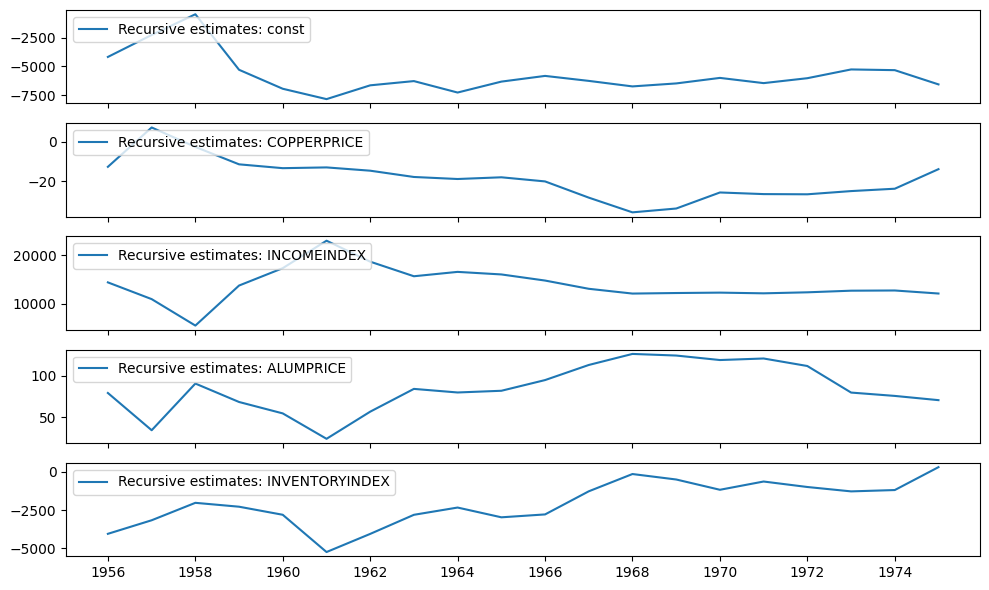
再帰係数は recursive_coefficients 属性で使用できます。または、 plot_recursive_coefficient メソッドを使用してプロットを生成することもできます。
[4]:
print(res.recursive_coefficients.filtered[0])
res.plot_recursive_coefficient(range(mod.k_exog), alpha=None, figsize=(10, 6))
[     2.88890087      4.94795049   1558.41803044   1958.43326658
 -51474.9578655   -4168.94974192  -2252.61351128   -446.55908507
  -5288.39794736  -6942.31935786  -7846.0890355   -6643.15121393
  -6274.11015558  -7272.01696292  -6319.02648554  -5822.23929148
  -6256.30902754  -6737.4044603   -6477.42841448  -5995.90746904
  -6450.80677813  -6022.92166487  -5258.35152753  -5320.89136363
  -6562.37193573]
[4]:

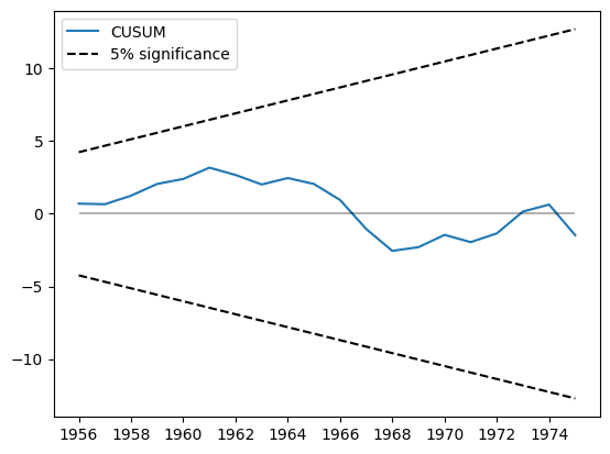
CUSUM統計量はcusum属性で利用できますが、通常はplot_cusumメソッドを使用してパラメータの安定性を視覚的に確認する方が便利です。下のプロットでは、CUSUM統計量が5%の有意水準帯を超えていないため、5%の水準で安定したパラメータの帰無仮説を棄却できません。
[5]:
print(res.cusum)
fig = res.plot_cusum()
[ 0.69971508  0.65841244  1.24629674  2.05476032  2.39888918  3.1786198
  2.67244672  2.01783215  2.46131747  2.05268638  0.95054336 -1.04505546
 -2.55465286 -2.29908152 -1.45289492 -1.95353993 -1.3504662   0.15789829
  0.6328653  -1.48184586]
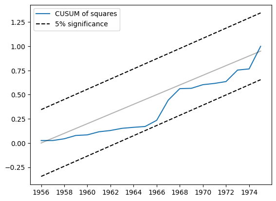
もう一つ関連する統計量は、二乗和のCUSUMです。これはcusum_squares属性で確認できますが、視覚的に確認する方が便利であり、そのためにplot_cusum_squaresメソッドが用意されています。以下のプロットでは、二乗和のCUSUM統計量は5%の有意水準バンドの外に出ていないため、5%の有意水準で安定したパラメータの帰無仮説を棄却できません。
[6]:
res.plot_cusum_squares()
[6]:

例2: 貨幣数量説
貨幣数量説は、「貨幣供給量の変化率の変化が与えられた場合、それは…物価上昇率の変化と等しい変化を引き起こす」と示唆しています(Lucas, 1980)。Lucasに従い、私たちは貨幣成長の両面指数加重移動平均とCPIインフレ率との関係を調べます。Lucasはこれらの変数間の関係が安定していることを発見しましたが、最近ではこの関係が不安定であるようです。例えば、SargentとSurico(2010)を参照してください。
[7]:
start = "1959-12-01"
end = "2015-01-01"
m2 = DataReader("M2SL", "fred", start=start, end=end)
cpi = DataReader("CPIAUCSL", "fred", start=start, end=end)
[8]:
def ewma(series, beta, n_window):
    nobs = len(series)
    scalar = (1 - beta) / (1 + beta)
    ma = []
    k = np.arange(n_window, 0, -1)
    weights = np.r_[beta ** k, 1, beta ** k[::-1]]
    for t in range(n_window, nobs - n_window):
        window = series.iloc[t - n_window : t + n_window + 1].values
        ma.append(scalar * np.sum(weights * window))
    return pd.Series(ma, name=series.name, index=series.iloc[n_window:-n_window].index)


m2_ewma = ewma(np.log(m2["M2SL"].resample("QS").mean()).diff().iloc[1:], 0.95, 10 * 4)
cpi_ewma = ewma(
    np.log(cpi["CPIAUCSL"].resample("QS").mean()).diff().iloc[1:], 0.95, 10 * 4
)
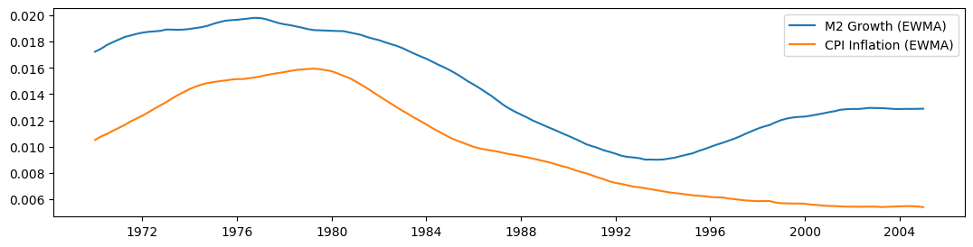
ルーカスの\(\beta = 0.95\)フィルター(両側に10年のウィンドウを使用)を使って移動平均を構築した後、以下に各シリーズをプロットします。サンプルの一部ではそれらが一緒に動いているように見えますが、1990年以降はそれらが分岐しているように見えます。
[9]:
fig, ax = plt.subplots(figsize=(13, 3))

ax.plot(m2_ewma, label="M2 Growth (EWMA)")
ax.plot(cpi_ewma, label="CPI Inflation (EWMA)")
ax.legend()
[9]:
<matplotlib.legend.Legend at 0x246e0a5ff10>
[10]:
endog = cpi_ewma
exog = sm.add_constant(m2_ewma)
exog.columns = ["const", "M2"]

mod = sm.RecursiveLS(endog, exog)
res = mod.fit()

print(res.summary())
                           Statespace Model Results
==============================================================================
Dep. Variable:               CPIAUCSL   No. Observations:                  141
Model:                    RecursiveLS   Log Likelihood                 692.328
Date:                Thu, 28 Nov 2024   R-squared:                       0.812
Time:                        23:11:20   AIC                          -1380.656
Sample:                    01-01-1970   BIC                          -1374.758
                         - 01-01-2005   HQIC                         -1378.259
Covariance Type:            nonrobust   Scale                            0.000
==============================================================================
                 coef    std err          z      P>|z|      [0.025      0.975]
------------------------------------------------------------------------------
const         -0.0034      0.001     -6.002      0.000      -0.004      -0.002
M2             0.9133      0.037     24.482      0.000       0.840       0.986
===================================================================================
Ljung-Box (L1) (Q):                 138.24   Jarque-Bera (JB):                18.28
Prob(Q):                              0.00   Prob(JB):                         0.00
Heteroskedasticity (H):               5.36   Skew:                            -0.81
Prob(H) (two-sided):                  0.00   Kurtosis:                         2.28
===================================================================================

Warnings:
[1] Parameters and covariance matrix estimates are RLS estimates conditional on the entire sample.
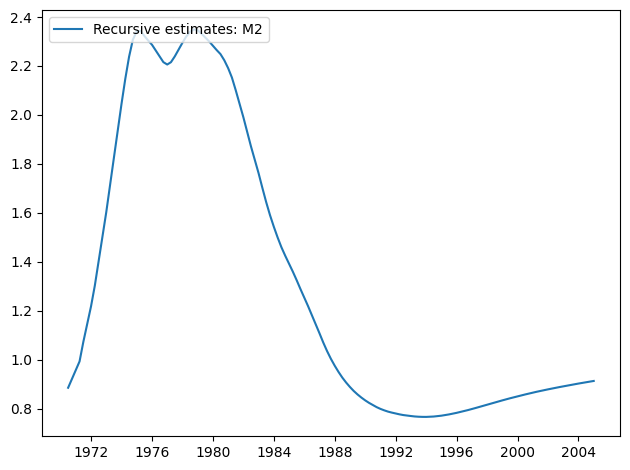
[11]:
res.plot_recursive_coefficient(1, alpha=None)
[11]:

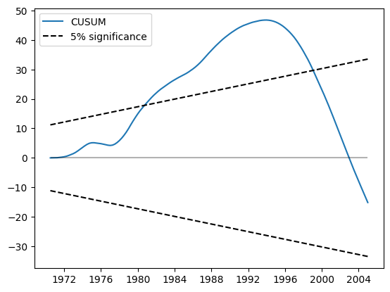
CUSUM プロットは 5% レベルで大幅な偏差を示しており、パラメータ安定性の帰無仮説が棄却されたことを示しています。
[12]:
res.plot_cusum()
[12]:

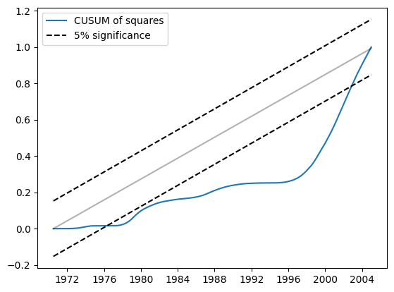
同様に、二乗の CUSUM は 5% レベルで大幅な偏差を示しており、これもパラメータ安定性の帰無仮説が棄却されることを示唆しています。
[13]:
res.plot_cusum_squares()
[13]:

例3: 線形制約と式
線形制約
モデルを構築する際に、constraintsパラメータを使用することで、線形制約を実装することは難しくありません。
[14]:
endog = dta["WORLDCONSUMPTION"]
exog = sm.add_constant(
    dta[["COPPERPRICE", "INCOMEINDEX", "ALUMPRICE", "INVENTORYINDEX"]]
)

mod = sm.RecursiveLS(endog, exog, constraints="COPPERPRICE = ALUMPRICE")
res = mod.fit()
print(res.summary())
                           Statespace Model Results
==============================================================================
Dep. Variable:       WORLDCONSUMPTION   No. Observations:                   25
Model:                    RecursiveLS   Log Likelihood                -134.231
Date:                Thu, 28 Nov 2024   R-squared:                       0.989
Time:                        23:11:23   AIC                            276.462
Sample:                    01-01-1951   BIC                            281.338
                         - 01-01-1975   HQIC                           277.814
Covariance Type:            nonrobust   Scale                       137155.014
==================================================================================
                     coef    std err          z      P>|z|      [0.025      0.975]
----------------------------------------------------------------------------------
const          -4839.4836   2412.410     -2.006      0.045   -9567.721    -111.246
COPPERPRICE        5.9797     12.704      0.471      0.638     -18.921      30.880
INCOMEINDEX     1.115e+04    666.308     16.738      0.000    9847.000    1.25e+04
ALUMPRICE          5.9797     12.704      0.471      0.638     -18.921      30.880
INVENTORYINDEX   241.3452   2298.951      0.105      0.916   -4264.515    4747.206
===================================================================================
Ljung-Box (L1) (Q):                   6.27   Jarque-Bera (JB):                 1.78
Prob(Q):                              0.01   Prob(JB):                         0.41
Heteroskedasticity (H):               1.75   Skew:                            -0.63
Prob(H) (two-sided):                  0.48   Kurtosis:                         2.32
===================================================================================

Warnings:
[1] Parameters and covariance matrix estimates are RLS estimates conditional on the entire sample.
式
同じモデルをクラスメソッドfrom_formulaを使ってフィットさせることができます。
[15]:
mod = sm.RecursiveLS.from_formula(
    "WORLDCONSUMPTION ~ COPPERPRICE + INCOMEINDEX + ALUMPRICE + INVENTORYINDEX",
    dta,
    constraints="COPPERPRICE = ALUMPRICE",
)
res = mod.fit()
print(res.summary())
                           Statespace Model Results
==============================================================================
Dep. Variable:       WORLDCONSUMPTION   No. Observations:                   25
Model:                    RecursiveLS   Log Likelihood                -134.231
Date:                Thu, 28 Nov 2024   R-squared:                       0.989
Time:                        23:11:23   AIC                            276.462
Sample:                    01-01-1951   BIC                            281.338
                         - 01-01-1975   HQIC                           277.814
Covariance Type:            nonrobust   Scale                       137155.014
==================================================================================
                     coef    std err          z      P>|z|      [0.025      0.975]
----------------------------------------------------------------------------------
Intercept      -4839.4836   2412.410     -2.006      0.045   -9567.721    -111.246
COPPERPRICE        5.9797     12.704      0.471      0.638     -18.921      30.880
INCOMEINDEX     1.115e+04    666.308     16.738      0.000    9847.000    1.25e+04
ALUMPRICE          5.9797     12.704      0.471      0.638     -18.921      30.880
INVENTORYINDEX   241.3452   2298.951      0.105      0.916   -4264.515    4747.206
===================================================================================
Ljung-Box (L1) (Q):                   6.27   Jarque-Bera (JB):                 1.78
Prob(Q):                              0.01   Prob(JB):                         0.41
Heteroskedasticity (H):               1.75   Skew:                            -0.63
Prob(H) (two-sided):                  0.48   Kurtosis:                         2.32
===================================================================================

Warnings:
[1] Parameters and covariance matrix estimates are RLS estimates conditional on the entire sample.
C:\Users\user\projects\statsmodels-main\statsmodels\tsa\base\tsa_model.py:465: ValueWarning: No frequency information was provided, so inferred frequency YS-JAN will be used.
  self._init_dates(dates, freq)