時系列モデルにおける決定論的項
[1]:
import matplotlib.pyplot as plt
import numpy as np
import pandas as pd

plt.rc("figure", figsize=(16, 9))
plt.rc("font", size=16)
基本的な使い方
基本的な設定は、DeterministicProcess を使用して直接構築できます。これには、定数、任意の次数の時間トレンド、季節成分またはフーリエ成分が含まれます。
このプロセスには、インデックスが必要で、これは標本全部(または標本内)のインデックスです。
まず、定数、線形の時間トレンド、および5期間の季節項を持つ決定論的プロセスを初期化します。in_sample メソッドは、インデックスに一致する値のフルセットを返します。
[2]:
from statsmodels.tsa.deterministic import DeterministicProcess

index = pd.RangeIndex(0, 100)
det_proc = DeterministicProcess(index, constant=True, order=1, seasonal=True, period=5)
det_proc.in_sample()
[2]:
| const | trend | s(2,5) | s(3,5) | s(4,5) | s(5,5) | |
|---|---|---|---|---|---|---|
| 0 | 1.0 | 1.0 | 0.0 | 0.0 | 0.0 | 0.0 |
| 1 | 1.0 | 2.0 | 1.0 | 0.0 | 0.0 | 0.0 |
| 2 | 1.0 | 3.0 | 0.0 | 1.0 | 0.0 | 0.0 |
| 3 | 1.0 | 4.0 | 0.0 | 0.0 | 1.0 | 0.0 |
| 4 | 1.0 | 5.0 | 0.0 | 0.0 | 0.0 | 1.0 |
| ... | ... | ... | ... | ... | ... | ... |
| 95 | 1.0 | 96.0 | 0.0 | 0.0 | 0.0 | 0.0 |
| 96 | 1.0 | 97.0 | 1.0 | 0.0 | 0.0 | 0.0 |
| 97 | 1.0 | 98.0 | 0.0 | 1.0 | 0.0 | 0.0 |
| 98 | 1.0 | 99.0 | 0.0 | 0.0 | 1.0 | 0.0 |
| 99 | 1.0 | 100.0 | 0.0 | 0.0 | 0.0 | 1.0 |
100 rows × 6 columns
out_of_sampleは、標本内の終了後の次のstepsの値を返します。
[3]:
det_proc.out_of_sample(15)
[3]:
| const | trend | s(2,5) | s(3,5) | s(4,5) | s(5,5) | |
|---|---|---|---|---|---|---|
| 100 | 1.0 | 101.0 | 0.0 | 0.0 | 0.0 | 0.0 |
| 101 | 1.0 | 102.0 | 1.0 | 0.0 | 0.0 | 0.0 |
| 102 | 1.0 | 103.0 | 0.0 | 1.0 | 0.0 | 0.0 |
| 103 | 1.0 | 104.0 | 0.0 | 0.0 | 1.0 | 0.0 |
| 104 | 1.0 | 105.0 | 0.0 | 0.0 | 0.0 | 1.0 |
| 105 | 1.0 | 106.0 | 0.0 | 0.0 | 0.0 | 0.0 |
| 106 | 1.0 | 107.0 | 1.0 | 0.0 | 0.0 | 0.0 |
| 107 | 1.0 | 108.0 | 0.0 | 1.0 | 0.0 | 0.0 |
| 108 | 1.0 | 109.0 | 0.0 | 0.0 | 1.0 | 0.0 |
| 109 | 1.0 | 110.0 | 0.0 | 0.0 | 0.0 | 1.0 |
| 110 | 1.0 | 111.0 | 0.0 | 0.0 | 0.0 | 0.0 |
| 111 | 1.0 | 112.0 | 1.0 | 0.0 | 0.0 | 0.0 |
| 112 | 1.0 | 113.0 | 0.0 | 1.0 | 0.0 | 0.0 |
| 113 | 1.0 | 114.0 | 0.0 | 0.0 | 1.0 | 0.0 |
| 114 | 1.0 | 115.0 | 0.0 | 0.0 | 0.0 | 1.0 |
range(start, stop) は、標本内外を含む任意の範囲で決定論的な項を生成するためにも使用できます。
注記
インデックスが pandas の
DatetimeIndexまたはPeriodIndexの場合、startとstopは日付形式(文字列、例えば 「2020-06-01」 や Timestamp)または整数を指定できます。stopは範囲に常に含まれます。これは Python らしくないかもしれませんが、statsmodels や Pandas が日付形式のスライスを扱う際にstopを含める必要があるためです。
[4]:
det_proc.range(190, 210)
[4]:
| const | trend | s(2,5) | s(3,5) | s(4,5) | s(5,5) | |
|---|---|---|---|---|---|---|
| 190 | 1.0 | 191.0 | 0.0 | 0.0 | 0.0 | 0.0 |
| 191 | 1.0 | 192.0 | 1.0 | 0.0 | 0.0 | 0.0 |
| 192 | 1.0 | 193.0 | 0.0 | 1.0 | 0.0 | 0.0 |
| 193 | 1.0 | 194.0 | 0.0 | 0.0 | 1.0 | 0.0 |
| 194 | 1.0 | 195.0 | 0.0 | 0.0 | 0.0 | 1.0 |
| 195 | 1.0 | 196.0 | 0.0 | 0.0 | 0.0 | 0.0 |
| 196 | 1.0 | 197.0 | 1.0 | 0.0 | 0.0 | 0.0 |
| 197 | 1.0 | 198.0 | 0.0 | 1.0 | 0.0 | 0.0 |
| 198 | 1.0 | 199.0 | 0.0 | 0.0 | 1.0 | 0.0 |
| 199 | 1.0 | 200.0 | 0.0 | 0.0 | 0.0 | 1.0 |
| 200 | 1.0 | 201.0 | 0.0 | 0.0 | 0.0 | 0.0 |
| 201 | 1.0 | 202.0 | 1.0 | 0.0 | 0.0 | 0.0 |
| 202 | 1.0 | 203.0 | 0.0 | 1.0 | 0.0 | 0.0 |
| 203 | 1.0 | 204.0 | 0.0 | 0.0 | 1.0 | 0.0 |
| 204 | 1.0 | 205.0 | 0.0 | 0.0 | 0.0 | 1.0 |
| 205 | 1.0 | 206.0 | 0.0 | 0.0 | 0.0 | 0.0 |
| 206 | 1.0 | 207.0 | 1.0 | 0.0 | 0.0 | 0.0 |
| 207 | 1.0 | 208.0 | 0.0 | 1.0 | 0.0 | 0.0 |
| 208 | 1.0 | 209.0 | 0.0 | 0.0 | 1.0 | 0.0 |
| 209 | 1.0 | 210.0 | 0.0 | 0.0 | 0.0 | 1.0 |
| 210 | 1.0 | 211.0 | 0.0 | 0.0 | 0.0 | 0.0 |
日付類似のインデックスを使用する
次に、PeriodIndex を使用して同じ手順を示します。
[5]:
index = pd.period_range("2020-03-01", freq="M", periods=60)
det_proc = DeterministicProcess(index, constant=True, fourier=2)
det_proc.in_sample().head(12)
[5]:
| const | sin(1,12) | cos(1,12) | sin(2,12) | cos(2,12) | |
|---|---|---|---|---|---|
| 2020-03 | 1.0 | 0.000000e+00 | 1.000000e+00 | 0.000000e+00 | 1.0 |
| 2020-04 | 1.0 | 5.000000e-01 | 8.660254e-01 | 8.660254e-01 | 0.5 |
| 2020-05 | 1.0 | 8.660254e-01 | 5.000000e-01 | 8.660254e-01 | -0.5 |
| 2020-06 | 1.0 | 1.000000e+00 | 6.123234e-17 | 1.224647e-16 | -1.0 |
| 2020-07 | 1.0 | 8.660254e-01 | -5.000000e-01 | -8.660254e-01 | -0.5 |
| 2020-08 | 1.0 | 5.000000e-01 | -8.660254e-01 | -8.660254e-01 | 0.5 |
| 2020-09 | 1.0 | 1.224647e-16 | -1.000000e+00 | -2.449294e-16 | 1.0 |
| 2020-10 | 1.0 | -5.000000e-01 | -8.660254e-01 | 8.660254e-01 | 0.5 |
| 2020-11 | 1.0 | -8.660254e-01 | -5.000000e-01 | 8.660254e-01 | -0.5 |
| 2020-12 | 1.0 | -1.000000e+00 | -1.836970e-16 | 3.673940e-16 | -1.0 |
| 2021-01 | 1.0 | -8.660254e-01 | 5.000000e-01 | -8.660254e-01 | -0.5 |
| 2021-02 | 1.0 | -5.000000e-01 | 8.660254e-01 | -8.660254e-01 | 0.5 |
[6]:
det_proc.out_of_sample(12)
[6]:
| const | sin(1,12) | cos(1,12) | sin(2,12) | cos(2,12) | |
|---|---|---|---|---|---|
| 2025-03 | 1.0 | -1.224647e-15 | 1.000000e+00 | -2.449294e-15 | 1.0 |
| 2025-04 | 1.0 | 5.000000e-01 | 8.660254e-01 | 8.660254e-01 | 0.5 |
| 2025-05 | 1.0 | 8.660254e-01 | 5.000000e-01 | 8.660254e-01 | -0.5 |
| 2025-06 | 1.0 | 1.000000e+00 | -4.904777e-16 | -9.809554e-16 | -1.0 |
| 2025-07 | 1.0 | 8.660254e-01 | -5.000000e-01 | -8.660254e-01 | -0.5 |
| 2025-08 | 1.0 | 5.000000e-01 | -8.660254e-01 | -8.660254e-01 | 0.5 |
| 2025-09 | 1.0 | 4.899825e-15 | -1.000000e+00 | -9.799650e-15 | 1.0 |
| 2025-10 | 1.0 | -5.000000e-01 | -8.660254e-01 | 8.660254e-01 | 0.5 |
| 2025-11 | 1.0 | -8.660254e-01 | -5.000000e-01 | 8.660254e-01 | -0.5 |
| 2025-12 | 1.0 | -1.000000e+00 | -3.184701e-15 | 6.369401e-15 | -1.0 |
| 2026-01 | 1.0 | -8.660254e-01 | 5.000000e-01 | -8.660254e-01 | -0.5 |
| 2026-02 | 1.0 | -5.000000e-01 | 8.660254e-01 | -8.660254e-01 | 0.5 |
range は日付のような引数を受け入れますが、通常は文字列として渡されます。
[7]:
det_proc.range("2025-01", "2026-01")
[7]:
| const | sin(1,12) | cos(1,12) | sin(2,12) | cos(2,12) | |
|---|---|---|---|---|---|
| 2025-01 | 1.0 | -8.660254e-01 | 5.000000e-01 | -8.660254e-01 | -0.5 |
| 2025-02 | 1.0 | -5.000000e-01 | 8.660254e-01 | -8.660254e-01 | 0.5 |
| 2025-03 | 1.0 | -1.224647e-15 | 1.000000e+00 | -2.449294e-15 | 1.0 |
| 2025-04 | 1.0 | 5.000000e-01 | 8.660254e-01 | 8.660254e-01 | 0.5 |
| 2025-05 | 1.0 | 8.660254e-01 | 5.000000e-01 | 8.660254e-01 | -0.5 |
| 2025-06 | 1.0 | 1.000000e+00 | -4.904777e-16 | -9.809554e-16 | -1.0 |
| 2025-07 | 1.0 | 8.660254e-01 | -5.000000e-01 | -8.660254e-01 | -0.5 |
| 2025-08 | 1.0 | 5.000000e-01 | -8.660254e-01 | -8.660254e-01 | 0.5 |
| 2025-09 | 1.0 | 4.899825e-15 | -1.000000e+00 | -9.799650e-15 | 1.0 |
| 2025-10 | 1.0 | -5.000000e-01 | -8.660254e-01 | 8.660254e-01 | 0.5 |
| 2025-11 | 1.0 | -8.660254e-01 | -5.000000e-01 | 8.660254e-01 | -0.5 |
| 2025-12 | 1.0 | -1.000000e+00 | -3.184701e-15 | 6.369401e-15 | -1.0 |
| 2026-01 | 1.0 | -8.660254e-01 | 5.000000e-01 | -8.660254e-01 | -0.5 |
これは、整数値58と70を使用することと同じです。
[8]:
det_proc.range(58, 70)
[8]:
| const | sin(1,12) | cos(1,12) | sin(2,12) | cos(2,12) | |
|---|---|---|---|---|---|
| 2025-01 | 1.0 | -8.660254e-01 | 5.000000e-01 | -8.660254e-01 | -0.5 |
| 2025-02 | 1.0 | -5.000000e-01 | 8.660254e-01 | -8.660254e-01 | 0.5 |
| 2025-03 | 1.0 | -1.224647e-15 | 1.000000e+00 | -2.449294e-15 | 1.0 |
| 2025-04 | 1.0 | 5.000000e-01 | 8.660254e-01 | 8.660254e-01 | 0.5 |
| 2025-05 | 1.0 | 8.660254e-01 | 5.000000e-01 | 8.660254e-01 | -0.5 |
| 2025-06 | 1.0 | 1.000000e+00 | -4.904777e-16 | -9.809554e-16 | -1.0 |
| 2025-07 | 1.0 | 8.660254e-01 | -5.000000e-01 | -8.660254e-01 | -0.5 |
| 2025-08 | 1.0 | 5.000000e-01 | -8.660254e-01 | -8.660254e-01 | 0.5 |
| 2025-09 | 1.0 | 4.899825e-15 | -1.000000e+00 | -9.799650e-15 | 1.0 |
| 2025-10 | 1.0 | -5.000000e-01 | -8.660254e-01 | 8.660254e-01 | 0.5 |
| 2025-11 | 1.0 | -8.660254e-01 | -5.000000e-01 | 8.660254e-01 | -0.5 |
| 2025-12 | 1.0 | -1.000000e+00 | -3.184701e-15 | 6.369401e-15 | -1.0 |
| 2026-01 | 1.0 | -8.660254e-01 | 5.000000e-01 | -8.660254e-01 | -0.5 |
高度な構築
コンストラクタで直接サポートされていない特徴を持つ決定論的プロセスは、additional_termsを使用して作成できます。この引数はDetermisticTermのリストを受け入れます。ここでは、2つの季節要素を持つ決定論的プロセスを作成します:5日周期の曜日成分と、365.25日の周期でフーリエ成分を通じて捕らえた年次成分です。
[9]:
from statsmodels.tsa.deterministic import Fourier, Seasonality, TimeTrend

index = pd.period_range("2020-03-01", freq="D", periods=2 * 365)
tt = TimeTrend(constant=True)
four = Fourier(period=365.25, order=2)
seas = Seasonality(period=7)
det_proc = DeterministicProcess(index, additional_terms=[tt, seas, four])
det_proc.in_sample().head(28)
[9]:
| const | s(2,7) | s(3,7) | s(4,7) | s(5,7) | s(6,7) | s(7,7) | sin(1,365.25) | cos(1,365.25) | sin(2,365.25) | cos(2,365.25) | |
|---|---|---|---|---|---|---|---|---|---|---|---|
| 2020-03-01 | 1.0 | 0.0 | 0.0 | 0.0 | 0.0 | 0.0 | 0.0 | 0.000000 | 1.000000 | 0.000000 | 1.000000 |
| 2020-03-02 | 1.0 | 1.0 | 0.0 | 0.0 | 0.0 | 0.0 | 0.0 | 0.017202 | 0.999852 | 0.034398 | 0.999408 |
| 2020-03-03 | 1.0 | 0.0 | 1.0 | 0.0 | 0.0 | 0.0 | 0.0 | 0.034398 | 0.999408 | 0.068755 | 0.997634 |
| 2020-03-04 | 1.0 | 0.0 | 0.0 | 1.0 | 0.0 | 0.0 | 0.0 | 0.051584 | 0.998669 | 0.103031 | 0.994678 |
| 2020-03-05 | 1.0 | 0.0 | 0.0 | 0.0 | 1.0 | 0.0 | 0.0 | 0.068755 | 0.997634 | 0.137185 | 0.990545 |
| 2020-03-06 | 1.0 | 0.0 | 0.0 | 0.0 | 0.0 | 1.0 | 0.0 | 0.085906 | 0.996303 | 0.171177 | 0.985240 |
| 2020-03-07 | 1.0 | 0.0 | 0.0 | 0.0 | 0.0 | 0.0 | 1.0 | 0.103031 | 0.994678 | 0.204966 | 0.978769 |
| 2020-03-08 | 1.0 | 0.0 | 0.0 | 0.0 | 0.0 | 0.0 | 0.0 | 0.120126 | 0.992759 | 0.238513 | 0.971139 |
| 2020-03-09 | 1.0 | 1.0 | 0.0 | 0.0 | 0.0 | 0.0 | 0.0 | 0.137185 | 0.990545 | 0.271777 | 0.962360 |
| 2020-03-10 | 1.0 | 0.0 | 1.0 | 0.0 | 0.0 | 0.0 | 0.0 | 0.154204 | 0.988039 | 0.304719 | 0.952442 |
| 2020-03-11 | 1.0 | 0.0 | 0.0 | 1.0 | 0.0 | 0.0 | 0.0 | 0.171177 | 0.985240 | 0.337301 | 0.941397 |
| 2020-03-12 | 1.0 | 0.0 | 0.0 | 0.0 | 1.0 | 0.0 | 0.0 | 0.188099 | 0.982150 | 0.369484 | 0.929237 |
| 2020-03-13 | 1.0 | 0.0 | 0.0 | 0.0 | 0.0 | 1.0 | 0.0 | 0.204966 | 0.978769 | 0.401229 | 0.915978 |
| 2020-03-14 | 1.0 | 0.0 | 0.0 | 0.0 | 0.0 | 0.0 | 1.0 | 0.221772 | 0.975099 | 0.432499 | 0.901634 |
| 2020-03-15 | 1.0 | 0.0 | 0.0 | 0.0 | 0.0 | 0.0 | 0.0 | 0.238513 | 0.971139 | 0.463258 | 0.886224 |
| 2020-03-16 | 1.0 | 1.0 | 0.0 | 0.0 | 0.0 | 0.0 | 0.0 | 0.255182 | 0.966893 | 0.493468 | 0.869764 |
| 2020-03-17 | 1.0 | 0.0 | 1.0 | 0.0 | 0.0 | 0.0 | 0.0 | 0.271777 | 0.962360 | 0.523094 | 0.852275 |
| 2020-03-18 | 1.0 | 0.0 | 0.0 | 1.0 | 0.0 | 0.0 | 0.0 | 0.288291 | 0.957543 | 0.552101 | 0.833777 |
| 2020-03-19 | 1.0 | 0.0 | 0.0 | 0.0 | 1.0 | 0.0 | 0.0 | 0.304719 | 0.952442 | 0.580455 | 0.814292 |
| 2020-03-20 | 1.0 | 0.0 | 0.0 | 0.0 | 0.0 | 1.0 | 0.0 | 0.321058 | 0.947060 | 0.608121 | 0.793844 |
| 2020-03-21 | 1.0 | 0.0 | 0.0 | 0.0 | 0.0 | 0.0 | 1.0 | 0.337301 | 0.941397 | 0.635068 | 0.772456 |
| 2020-03-22 | 1.0 | 0.0 | 0.0 | 0.0 | 0.0 | 0.0 | 0.0 | 0.353445 | 0.935455 | 0.661263 | 0.750154 |
| 2020-03-23 | 1.0 | 1.0 | 0.0 | 0.0 | 0.0 | 0.0 | 0.0 | 0.369484 | 0.929237 | 0.686676 | 0.726964 |
| 2020-03-24 | 1.0 | 0.0 | 1.0 | 0.0 | 0.0 | 0.0 | 0.0 | 0.385413 | 0.922744 | 0.711276 | 0.702913 |
| 2020-03-25 | 1.0 | 0.0 | 0.0 | 1.0 | 0.0 | 0.0 | 0.0 | 0.401229 | 0.915978 | 0.735034 | 0.678031 |
| 2020-03-26 | 1.0 | 0.0 | 0.0 | 0.0 | 1.0 | 0.0 | 0.0 | 0.416926 | 0.908940 | 0.757922 | 0.652346 |
| 2020-03-27 | 1.0 | 0.0 | 0.0 | 0.0 | 0.0 | 1.0 | 0.0 | 0.432499 | 0.901634 | 0.779913 | 0.625889 |
| 2020-03-28 | 1.0 | 0.0 | 0.0 | 0.0 | 0.0 | 0.0 | 1.0 | 0.447945 | 0.894061 | 0.800980 | 0.598691 |
カスタム決定論的項目
DetermisticTerm 抽象基底クラスは、ユーザーがカスタム決定論的項目を書くのを助けるためにサブクラス化するように設計されています。次に、2つの例を示します。1つ目は、一定の期間数後に分割できる時間トレンドです。2つ目は、「トリック」決定論的項目で、外生データ(実際には決定論的プロセスではないもの)を決定論的なものとして扱うことができるようにします。これにより、予測に必要な項目を収集する際の簡素化が可能になります。
これらはカスタム項目の構築を示すことを目的としています。入力検証の面で改善の余地は確実にあります。
[10]:
from statsmodels.tsa.deterministic import DeterministicTerm


class BrokenTimeTrend(DeterministicTerm):
    def __init__(self, break_period: int):
        self._break_period = break_period

    def __str__(self):
        return "Broken Time Trend"

    def _eq_attr(self):
        return (self._break_period,)

    def in_sample(self, index: pd.Index):
        nobs = index.shape[0]
        terms = np.zeros((nobs, 2))
        terms[self._break_period :, 0] = 1
        terms[self._break_period :, 1] = np.arange(self._break_period + 1, nobs + 1)
        return pd.DataFrame(terms, columns=["const_break", "trend_break"], index=index)

    def out_of_sample(
        self, steps: int, index: pd.Index, forecast_index: pd.Index = None
    ):
        # Always call extend index first
        fcast_index = self._extend_index(index, steps, forecast_index)
        nobs = index.shape[0]
        terms = np.zeros((steps, 2))
        # Assume break period is in-sample
        terms[:, 0] = 1
        terms[:, 1] = np.arange(nobs + 1, nobs + steps + 1)
        return pd.DataFrame(
            terms, columns=["const_break", "trend_break"], index=fcast_index
        )
[11]:
btt = BrokenTimeTrend(60)
tt = TimeTrend(constant=True, order=1)
index = pd.RangeIndex(100)
det_proc = DeterministicProcess(index, additional_terms=[tt, btt])
det_proc.range(55, 65)
[11]:
| const | trend | const_break | trend_break | |
|---|---|---|---|---|
| 55 | 1.0 | 56.0 | 0.0 | 0.0 |
| 56 | 1.0 | 57.0 | 0.0 | 0.0 |
| 57 | 1.0 | 58.0 | 0.0 | 0.0 |
| 58 | 1.0 | 59.0 | 0.0 | 0.0 |
| 59 | 1.0 | 60.0 | 0.0 | 0.0 |
| 60 | 1.0 | 61.0 | 1.0 | 61.0 |
| 61 | 1.0 | 62.0 | 1.0 | 62.0 |
| 62 | 1.0 | 63.0 | 1.0 | 63.0 |
| 63 | 1.0 | 64.0 | 1.0 | 64.0 |
| 64 | 1.0 | 65.0 | 1.0 | 65.0 |
| 65 | 1.0 | 66.0 | 1.0 | 66.0 |
次に、予測のために標本外の外生変数配列を構築する際に簡単にできるよう、実際の外生データに対する簡単な「ラッパー」を作成します。
[12]:
class ExogenousProcess(DeterministicTerm):
    def __init__(self, data):
        self._data = data

    def __str__(self):
        return "Custom Exog Process"

    def _eq_attr(self):
        return (id(self._data),)

    def in_sample(self, index: pd.Index):
        return self._data.loc[index]

    def out_of_sample(
        self, steps: int, index: pd.Index, forecast_index: pd.Index = None
    ):
        forecast_index = self._extend_index(index, steps, forecast_index)
        return self._data.loc[forecast_index]
[13]:
import numpy as np

gen = np.random.default_rng(98765432101234567890)
exog = pd.DataFrame(gen.integers(100, size=(300, 2)), columns=["exog1", "exog2"])
exog.head()
[13]:
| exog1 | exog2 | |
|---|---|---|
| 0 | 6 | 99 |
| 1 | 64 | 28 |
| 2 | 15 | 81 |
| 3 | 54 | 8 |
| 4 | 12 | 8 |
[14]:
ep = ExogenousProcess(exog)
tt = TimeTrend(constant=True, order=1)
# The in-sample index
idx = exog.index[:200]
det_proc = DeterministicProcess(idx, additional_terms=[tt, ep])
[15]:
det_proc.in_sample().head()
[15]:
| const | trend | exog1 | exog2 | |
|---|---|---|---|---|
| 0 | 1.0 | 1.0 | 6 | 99 |
| 1 | 1.0 | 2.0 | 64 | 28 |
| 2 | 1.0 | 3.0 | 15 | 81 |
| 3 | 1.0 | 4.0 | 54 | 8 |
| 4 | 1.0 | 5.0 | 12 | 8 |
[16]:
det_proc.out_of_sample(10)
[16]:
| const | trend | exog1 | exog2 | |
|---|---|---|---|---|
| 200 | 1.0 | 201.0 | 56 | 88 |
| 201 | 1.0 | 202.0 | 48 | 84 |
| 202 | 1.0 | 203.0 | 44 | 5 |
| 203 | 1.0 | 204.0 | 65 | 63 |
| 204 | 1.0 | 205.0 | 63 | 39 |
| 205 | 1.0 | 206.0 | 89 | 39 |
| 206 | 1.0 | 207.0 | 41 | 54 |
| 207 | 1.0 | 208.0 | 71 | 5 |
| 208 | 1.0 | 209.0 | 89 | 6 |
| 209 | 1.0 | 210.0 | 58 | 63 |
モデルサポート
DeterministicProcess を直接サポートするモデルは AutoReg のみです。カスタム項目は deterministic キーワード引数を使用して設定できます。
注意: カスタム項目を使用するには、trend="n" と seasonal=False を設定する必要があり、すべての決定論的成分はカスタム決定論的項目から来る必要があります。
データのシミュレーション
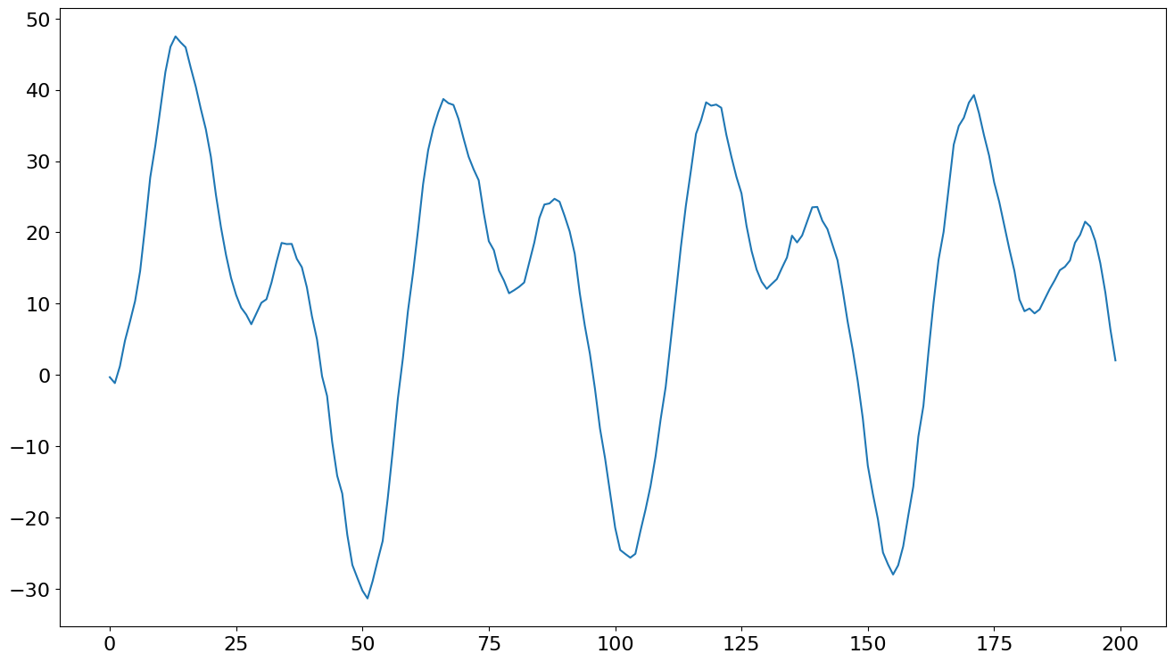
ここでは、フーリエ級数によって週次の季節性を捉えたデータをシミュレートします。
[17]:
gen = np.random.default_rng(98765432101234567890)
idx = pd.RangeIndex(200)
det_proc = DeterministicProcess(idx, constant=True, period=52, fourier=2)
det_terms = det_proc.in_sample().to_numpy()
params = np.array([1.0, 3, -1, 4, -2])
exog = det_terms @ params
y = np.empty(200)
y[0] = det_terms[0] @ params + gen.standard_normal()
for i in range(1, 200):
    y[i] = 0.9 * y[i - 1] + det_terms[i] @ params + gen.standard_normal()
y = pd.Series(y, index=idx)
ax = y.plot()
モデルは次に、deterministicキーワード引数を使ってフィットされます。seasonalはデフォルトでFalseですが、trendはデフォルトで"c"なので、これを変更する必要があります。
[18]:
from statsmodels.tsa.api import AutoReg

mod = AutoReg(y, 1, trend="n", deterministic=det_proc)
res = mod.fit()
print(res.summary())
                            AutoReg Model Results
==============================================================================
Dep. Variable:                      y   No. Observations:                  200
Model:                     AutoReg(1)   Log Likelihood                -270.964
Method:               Conditional MLE   S.D. of innovations              0.944
Date:                Thu, 28 Nov 2024   AIC                            555.927
Time:                        23:10:28   BIC                            578.980
Sample:                             1   HQIC                           565.258
                                  200
==============================================================================
                 coef    std err          z      P>|z|      [0.025      0.975]
------------------------------------------------------------------------------
const          0.8436      0.172      4.916      0.000       0.507       1.180
sin(1,52)      2.9738      0.160     18.587      0.000       2.660       3.287
cos(1,52)     -0.6771      0.284     -2.380      0.017      -1.235      -0.120
sin(2,52)      3.9951      0.099     40.336      0.000       3.801       4.189
cos(2,52)     -1.7206      0.264     -6.519      0.000      -2.238      -1.203
y.L1           0.9116      0.014     63.264      0.000       0.883       0.940
                                    Roots
=============================================================================
                  Real          Imaginary           Modulus         Frequency
-----------------------------------------------------------------------------
AR.1            1.0970           +0.0000j            1.0970            0.0000
-----------------------------------------------------------------------------
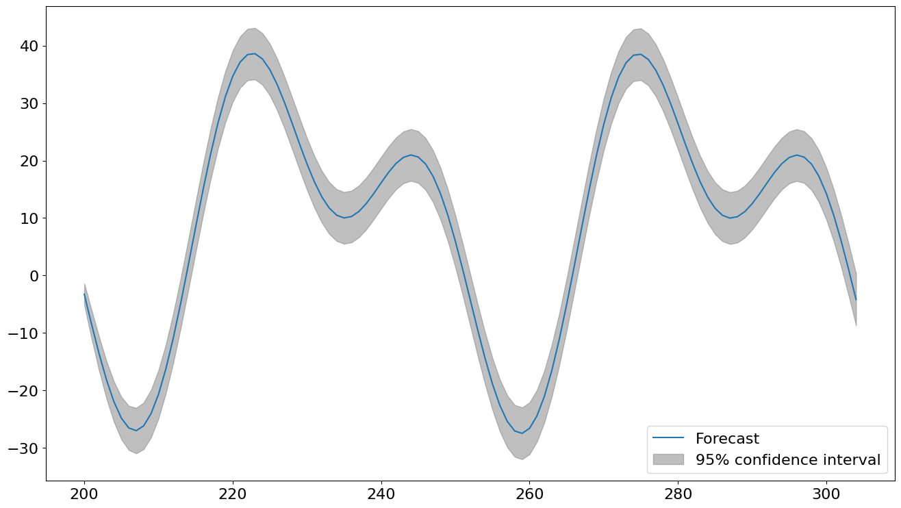
plot_predict を使用して、予測値とその予測区間を表示できます。標本外の決定論的な値は、AutoReg に渡された決定論的プロセスによって自動的に生成されます。
[19]:
fig = res.plot_predict(200, 200 + 2 * 52, True)
[20]:
auto_reg_forecast = res.predict(200, 211)
auto_reg_forecast
[20]:
200    -3.253482
201    -8.555660
202   -13.607557
203   -18.152622
204   -21.950370
205   -24.790116
206   -26.503171
207   -26.972781
208   -26.141244
209   -24.013773
210   -20.658891
211   -16.205310
dtype: float64
他のモデルとの併用
他のモデルはDeterministicProcessを直接サポートしていません。その代わりに、外生変数をサポートするモデルに任意の決定論的項を手動でexogとして渡すことができます。
SARIMAXと外生変数を使用する場合、これはSARIMA誤差を持つOLS(最小二乗法)であるため、モデルは次のように表現されます:
決定論的項のパラメータは、次の式に従って進化するAutoRegと直接比較することはできません:
もし\(x_t\)が決定論的項のみを含む場合、これら二つの表現は同等です(\(\theta(L)=0\)と仮定して、MA(移動平均項)が存在しない場合)。
[21]:
from statsmodels.tsa.api import SARIMAX

det_proc = DeterministicProcess(idx, period=52, fourier=2)
det_terms = det_proc.in_sample()

mod = SARIMAX(y, order=(1, 0, 0), trend="c", exog=det_terms)
res = mod.fit(disp=False)
print(res.summary())
                               SARIMAX Results
==============================================================================
Dep. Variable:                      y   No. Observations:                  200
Model:               SARIMAX(1, 0, 0)   Log Likelihood                -293.381
Date:                Thu, 28 Nov 2024   AIC                            600.763
Time:                        23:10:29   BIC                            623.851
Sample:                             0   HQIC                           610.106
                                - 200
Covariance Type:                  opg
==============================================================================
                 coef    std err          z      P>|z|      [0.025      0.975]
------------------------------------------------------------------------------
intercept      0.0797      0.140      0.567      0.570      -0.196       0.355
sin(1,52)      9.1916      0.876     10.492      0.000       7.475      10.909
cos(1,52)    -17.4348      0.891    -19.576      0.000     -19.180     -15.689
sin(2,52)      1.2512      0.466      2.683      0.007       0.337       2.165
cos(2,52)    -17.1863      0.434    -39.583      0.000     -18.037     -16.335
ar.L1          0.9957      0.007    150.762      0.000       0.983       1.009
sigma2         1.0748      0.119      9.068      0.000       0.842       1.307
===================================================================================
Ljung-Box (L1) (Q):                   2.16   Jarque-Bera (JB):                 1.03
Prob(Q):                              0.14   Prob(JB):                         0.60
Heteroskedasticity (H):               0.71   Skew:                            -0.14
Prob(H) (two-sided):                  0.16   Kurtosis:                         2.78
===================================================================================

Warnings:
[1] Covariance matrix calculated using the outer product of gradients (complex-step).
予測は似ていますが、SARIMAXのパラメータはMLE(最尤推定)を使用して推定されるのに対し、AutoRegはOLS(最小二乗法)を使用しているため異なります。
[22]:
sarimax_forecast = res.forecast(12, exog=det_proc.out_of_sample(12))
df = pd.concat([auto_reg_forecast, sarimax_forecast], axis=1)
df.columns = columns = ["AutoReg", "SARIMAX"]
df
[22]:
| AutoReg | SARIMAX | |
|---|---|---|
| 200 | -3.253482 | -2.956562 |
| 201 | -8.555660 | -7.985588 |
| 202 | -13.607557 | -12.794072 |
| 203 | -18.152622 | -17.130963 |
| 204 | -21.950370 | -20.760473 |
| 205 | -24.790116 | -23.475511 |
| 206 | -26.503171 | -25.109629 |
| 207 | -26.972781 | -25.546789 |
| 208 | -26.141244 | -24.728384 |
| 209 | -24.013773 | -22.657094 |
| 210 | -20.658891 | -19.397352 |
| 211 | -16.205310 | -15.072385 |