マルコフスイッチング自己回帰モデル¶

このノートブックでは、Kim and Nelson (1999)で示されたいくつかの結果を再現するために、statsmodelsのマルコフスイッチングモデルの使用例を提供します。Hamilton (1989) フィルターとKim (1994) スムーザーを適用しています。

これは、E-Views 8のマルコフスイッチングモデル（http://www.eviews.com/EViews8/ev8ecswitch_n.html#MarkovAR）や、Stata 14のマルコフスイッチングモデル（http://www.stata.com/manuals14/tsmswitch.pdf）と比較してテストされています。

[1]:

%matplotlib inline

from datetime import datetime
from io import BytesIO

import matplotlib.pyplot as plt
import numpy as np
import pandas as pd
import requests
import statsmodels.api as sm

# NBER recessions
from pandas_datareader.data import DataReader

usrec = DataReader(
    "USREC", "fred", start=datetime(1947, 1, 1), end=datetime(2013, 4, 1)
)

ハミルトン（1989）のGNPスイッチングモデル¶

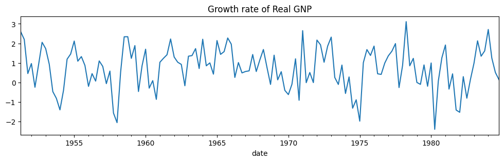
これは、マルコフスイッチングモデルを導入したハミルトン（1989）の画期的な論文を再現したものです。このモデルは、プロセスの平均が2つのレジーム間でスイッチする4次の自己回帰モデルです。次のように書くことができます。

\[y_t = \mu_{S_t} + \phi_1 (y_{t-1} - \mu_{S_{t-1}}) + \phi_2 (y_{t-2} - \mu_{S_{t-2}}) + \phi_3 (y_{t-3} - \mu_{S_{t-3}}) + \phi_4 (y_{t-4} - \mu_{S_{t-4}}) + \varepsilon_t\]

各期間において、レジームは以下の遷移確率行列に従って遷移します：

\[\begin{split} P(S_t = s_t | S_{t-1} = s_{t-1}) = \begin{bmatrix} p_{00} & p_{10} \\ p_{01} & p_{11} \end{bmatrix}\end{split}\]

ここで、\(p_{ij}\)はレジーム\(i\)からレジーム\(j\)への遷移確率を示します。

このモデルのクラスは、statsmodelsの時系列部分にあるMarkovAutoregressionです。モデルを作成するには、k_regimes=2でレジームの数を指定し、order=4で自己回帰の次数を指定する必要があります。デフォルトのモデルにはスイッチング自己回帰係数が含まれていますが、ここではswitching_ar=Falseを指定してそれを避けます。

作成後、モデルは最尤推定法でfitされます。内部では、期待値最大化（EM）アルゴリズムのいくつかのステップを使用して良い初期パラメータが見つけられ、クワジ・ニュートン（BFGS）アルゴリズムが適用されて最大値を素早く見つけます。

[2]:

# Get the RGNP data to replicate Hamilton
dta = pd.read_stata("rgnp.dta").iloc[1:]
dta.index = pd.DatetimeIndex(dta.date, freq="QS")
dta_hamilton = dta.rgnp

# Plot the data
dta_hamilton.plot(title="Growth rate of Real GNP", figsize=(12, 3))

# Fit the model
mod_hamilton = sm.tsa.MarkovAutoregression(
    dta_hamilton, k_regimes=2, order=4, switching_ar=False
)
res_hamilton = mod_hamilton.fit()

../../../_images/examples_notebooks_generated_markov_autoregression_4_0.png

[3]:

res_hamilton.summary()

[3]:

Markov Switching Model Results
Dep. Variable:	rgnp	No. Observations:	131
Model:	MarkovAutoregression	Log Likelihood	-181.263
Date:	Thu, 28 Nov 2024	AIC	380.527
Time:	23:10:50	BIC	406.404
Sample:	04-01-1951	HQIC	391.042
	- 10-01-1984
Covariance Type:	approx

Regime 0 parameters
	coef	std err	z	P>\|z\|	[0.025	0.975]
const	-0.3588	0.265	-1.356	0.175	-0.877	0.160

Regime 1 parameters
	coef	std err	z	P>\|z\|	[0.025	0.975]
const	1.1635	0.075	15.614	0.000	1.017	1.310

Non-switching parameters
	coef	std err	z	P>\|z\|	[0.025	0.975]
sigma2	0.5914	0.103	5.761	0.000	0.390	0.793
ar.L1	0.0135	0.120	0.112	0.911	-0.222	0.249
ar.L2	-0.0575	0.138	-0.418	0.676	-0.327	0.212
ar.L3	-0.2470	0.107	-2.310	0.021	-0.457	-0.037
ar.L4	-0.2129	0.111	-1.926	0.054	-0.430	0.004

Regime transition parameters
	coef	std err	z	P>\|z\|	[0.025	0.975]
p[0->0]	0.7547	0.097	7.819	0.000	0.565	0.944
p[1->0]	0.0959	0.038	2.542	0.011	0.022	0.170

Warnings:
[1] Covariance matrix calculated using numerical (complex-step) differentiation.

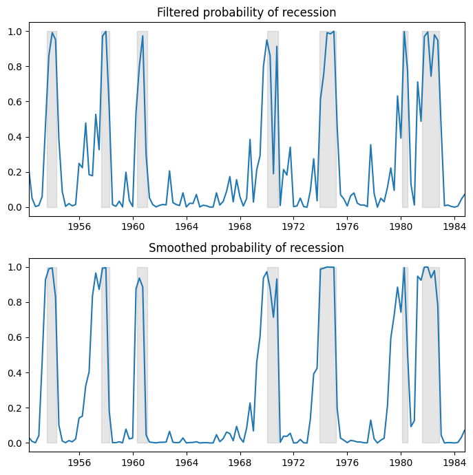
私たちは、景気後退の確率のフィルタリングおよびスムージングされた推定値をプロットします。フィルタリングとは、時刻 \(t\) における確率の推定値で、時刻 \(t\) までのデータに基づいています（ただし、時刻 \(t+1, ..., T\) のデータは除外されます）。スムージングとは、標本内のすべてのデータを使用して、時刻 \(t\) における確率の推定値を算出することを指します。

参考までに、灰色の期間はNBERの景気後退期間を示しています。

[4]:

fig, axes = plt.subplots(2, figsize=(7, 7))
ax = axes[0]
ax.plot(res_hamilton.filtered_marginal_probabilities[0])
ax.fill_between(usrec.index, 0, 1, where=usrec["USREC"].values, color="k", alpha=0.1)
ax.set_xlim(dta_hamilton.index[4], dta_hamilton.index[-1])
ax.set(title="Filtered probability of recession")

ax = axes[1]
ax.plot(res_hamilton.smoothed_marginal_probabilities[0])
ax.fill_between(usrec.index, 0, 1, where=usrec["USREC"].values, color="k", alpha=0.1)
ax.set_xlim(dta_hamilton.index[4], dta_hamilton.index[-1])
ax.set(title="Smoothed probability of recession")

fig.tight_layout()

../../../_images/examples_notebooks_generated_markov_autoregression_7_0.png

推定された遷移行列から、不況と拡張の予想期間を計算することができます。

[5]:

print(res_hamilton.expected_durations)

[ 4.07604745 10.42589385]

この場合、景気後退は約1年間（4四半期）、景気拡大は約2年半続くと予想されています。

Kim, Nelson, and Startz (1998) 三状態分散スイッチングモデル¶

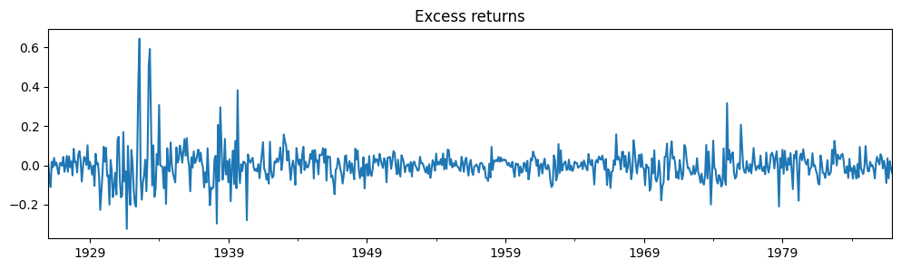
このモデルは、レジームの異方分散（分散の切り替え）を持ち、平均効果がない場合の推定を示しています。データセットは以下のリンクからアクセスできます： http://econ.korea.ac.kr/~cjkim/MARKOV/data/ew_excs.prn

対象となるモデルは次の通りです：

\[\begin{split}\begin{align} y_t & = \varepsilon_t \\ \varepsilon_t & \sim N(0, \sigma_{S_t}^2) \end{align}\end{split}\]

自己回帰成分がないため、このモデルは MarkovRegression クラスを使用して適合できます。平均効果がないため、trend='n' を指定します。分散が切り替わるレジームは3つであると仮定されているため、k_regimes=3 と switching_variance=True を指定します（デフォルトでは、レジーム間で分散は同じであると仮定されます）。

[6]:

# Get the dataset
ew_excs = requests.get("http://econ.korea.ac.kr/~cjkim/MARKOV/data/ew_excs.prn").content
raw = pd.read_table(BytesIO(ew_excs), header=None, skipfooter=1, engine="python")
raw.index = pd.date_range("1926-01-01", "1995-12-01", freq="MS")

dta_kns = raw.loc[:"1986"] - raw.loc[:"1986"].mean()

# Plot the dataset
dta_kns[0].plot(title="Excess returns", figsize=(12, 3))

# Fit the model
mod_kns = sm.tsa.MarkovRegression(
    dta_kns, k_regimes=3, trend="n", switching_variance=True
)
res_kns = mod_kns.fit()

../../../_images/examples_notebooks_generated_markov_autoregression_12_0.png

[7]:

res_kns.summary()

[7]:

Markov Switching Model Results
Dep. Variable:	0	No. Observations:	732
Model:	MarkovRegression	Log Likelihood	1001.895
Date:	Thu, 28 Nov 2024	AIC	-1985.790
Time:	23:10:57	BIC	-1944.428
Sample:	01-01-1926	HQIC	-1969.834
	- 12-01-1986
Covariance Type:	approx

Regime 0 parameters
	coef	std err	z	P>\|z\|	[0.025	0.975]
sigma2	0.0012	0.000	7.136	0.000	0.001	0.002

Regime 1 parameters
	coef	std err	z	P>\|z\|	[0.025	0.975]
sigma2	0.0040	0.000	8.489	0.000	0.003	0.005

Regime 2 parameters
	coef	std err	z	P>\|z\|	[0.025	0.975]
sigma2	0.0311	0.006	5.461	0.000	0.020	0.042

Regime transition parameters
	coef	std err	z	P>\|z\|	[0.025	0.975]
p[0->0]	0.9747	0.000	7857.416	0.000	0.974	0.975
p[1->0]	0.0195	0.010	1.949	0.051	-0.000	0.039
p[2->0]	2.354e-08	nan	nan	nan	nan	nan
p[0->1]	0.0253	3.97e-05	637.835	0.000	0.025	0.025
p[1->1]	0.9688	0.013	75.528	0.000	0.944	0.994
p[2->1]	0.0493	0.032	1.551	0.121	-0.013	0.112

Warnings:
[1] Covariance matrix calculated using numerical (complex-step) differentiation.

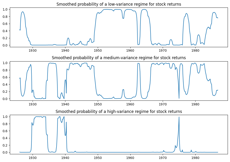
以下に、各レジームにいる確率をプロットします。高分散レジームが確率的に高いのは、いくつかの期間に限られます。

[8]:

fig, axes = plt.subplots(3, figsize=(10, 7))

ax = axes[0]
ax.plot(res_kns.smoothed_marginal_probabilities[0])
ax.set(title="Smoothed probability of a low-variance regime for stock returns")

ax = axes[1]
ax.plot(res_kns.smoothed_marginal_probabilities[1])
ax.set(title="Smoothed probability of a medium-variance regime for stock returns")

ax = axes[2]
ax.plot(res_kns.smoothed_marginal_probabilities[2])
ax.set(title="Smoothed probability of a high-variance regime for stock returns")

fig.tight_layout()

../../../_images/examples_notebooks_generated_markov_autoregression_15_0.png

フィラルド（1994年）の時間変動遷移確率¶

このモデルは、時間変動する遷移確率による推定を示しています。データセットは以下のリンクから取得できます: http://econ.korea.ac.kr/~cjkim/MARKOV/data/filardo.prn

上記のモデルでは、遷移確率が時間を通じて一定であると仮定していました。ここでは、遷移確率が経済の状態に応じて変化することを許容します。それ以外は、ハミルトン（1989年）のマルコフ自己回帰モデルと同様です。

各期間において、レジームは次の時間変動遷移確率の行列に従って遷移します:

\[\begin{split} P(S_t = s_t | S_{t-1} = s_{t-1}) = \begin{bmatrix} p_{00,t} & p_{10,t} \\ p_{01,t} & p_{11,t} \end{bmatrix}\end{split}\]

ここで、\(p_{ij,t}\) は、期間\(t\)においてレジーム\(i\)からレジーム\(j\)への遷移確率であり、次のように定義されます:

\[p_{ij,t} = \frac{\exp\{ x_{t-1}' \beta_{ij} \}}{1 + \exp\{ x_{t-1}' \beta_{ij} \}}\]

遷移確率を最尤推定の一部として推定する代わりに、回帰係数\(\beta_{ij}\)を推定します。これらの回帰係数は、遷移確率と、予め決定されたまたは外生的な回帰変数\(x_{t-1}\)との関係を示します。

[9]:

# Get the dataset
filardo = requests.get("http://econ.korea.ac.kr/~cjkim/MARKOV/data/filardo.prn").content
dta_filardo = pd.read_table(
    BytesIO(filardo), sep=" +", header=None, skipfooter=1, engine="python"
)
dta_filardo.columns = ["month", "ip", "leading"]
dta_filardo.index = pd.date_range("1948-01-01", "1991-04-01", freq="MS")

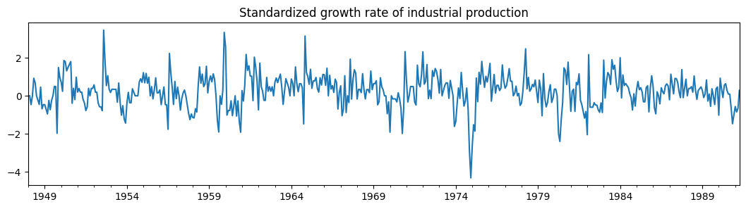
dta_filardo["dlip"] = np.log(dta_filardo["ip"]).diff() * 100
# Deflated pre-1960 observations by ratio of std. devs.
# See hmt_tvp.opt or Filardo (1994) p. 302
std_ratio = (
    dta_filardo["dlip"]["1960-01-01":].std() / dta_filardo["dlip"][:"1959-12-01"].std()
)
dta_filardo["dlip"][:"1959-12-01"] = dta_filardo["dlip"][:"1959-12-01"] * std_ratio

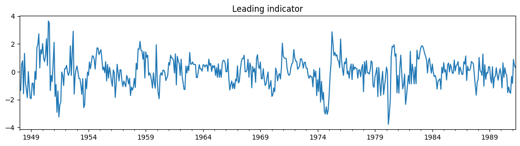
dta_filardo["dlleading"] = np.log(dta_filardo["leading"]).diff() * 100
dta_filardo["dmdlleading"] = dta_filardo["dlleading"] - dta_filardo["dlleading"].mean()

# Plot the data
dta_filardo["dlip"].plot(
    title="Standardized growth rate of industrial production", figsize=(13, 3)
)
plt.figure()
dta_filardo["dmdlleading"].plot(title="Leading indicator", figsize=(13, 3))

C:\Users\user\AppData\Local\Temp\ipykernel_13456\2507337649.py:15: FutureWarning: ChainedAssignmentError: behaviour will change in pandas 3.0!
You are setting values through chained assignment. Currently this works in certain cases, but when using Copy-on-Write (which will become the default behaviour in pandas 3.0) this will never work to update the original DataFrame or Series, because the intermediate object on which we are setting values will behave as a copy.
A typical example is when you are setting values in a column of a DataFrame, like:

df["col"][row_indexer] = value

Use `df.loc[row_indexer, "col"] = values` instead, to perform the assignment in a single step and ensure this keeps updating the original `df`.

See the caveats in the documentation: https://pandas.pydata.org/pandas-docs/stable/user_guide/indexing.html#returning-a-view-versus-a-copy

  dta_filardo["dlip"][:"1959-12-01"] = dta_filardo["dlip"][:"1959-12-01"] * std_ratio

[9]:

<Axes: title={'center': 'Leading indicator'}>

../../../_images/examples_notebooks_generated_markov_autoregression_17_2.png

../../../_images/examples_notebooks_generated_markov_autoregression_17_3.png

時間変動遷移確率は exog_tvtp パラメータによって指定されます。

ここでは、モデル適合の別の特徴を示します - MLEの初期パラメータを求めるためのランダムサーチの使用です。マルコフスイッチングモデルは、尤度関数の局所的な最大値が多く特徴であることがよくあるため、最適化の初期ステップを実行することが最良のパラメータを見つけるのに役立ちます。

以下では、初期パラメータベクトルから20個のランダムな摂動を調べ、最良のものを実際の初期パラメータとして使用することを指定します。検索がランダムであるため、結果の再現性を確保するために、事前に乱数生成器をシードします。

[10]:

mod_filardo = sm.tsa.MarkovAutoregression(
    dta_filardo.iloc[2:]["dlip"],
    k_regimes=2,
    order=4,
    switching_ar=False,
    exog_tvtp=sm.add_constant(dta_filardo.iloc[1:-1]["dmdlleading"]),
)

np.random.seed(12345)
res_filardo = mod_filardo.fit(search_reps=20)

[11]:

res_filardo.summary()

[11]:

Markov Switching Model Results
Dep. Variable:	dlip	No. Observations:	514
Model:	MarkovAutoregression	Log Likelihood	-586.572
Date:	Thu, 28 Nov 2024	AIC	1195.144
Time:	23:11:23	BIC	1241.808
Sample:	03-01-1948	HQIC	1213.433
	- 04-01-1991
Covariance Type:	approx

Regime 0 parameters
	coef	std err	z	P>\|z\|	[0.025	0.975]
const	-0.8659	0.153	-5.658	0.000	-1.166	-0.566

Regime 1 parameters
	coef	std err	z	P>\|z\|	[0.025	0.975]
const	0.5173	0.077	6.706	0.000	0.366	0.668

Non-switching parameters
	coef	std err	z	P>\|z\|	[0.025	0.975]
sigma2	0.4844	0.037	13.172	0.000	0.412	0.556
ar.L1	0.1895	0.050	3.761	0.000	0.091	0.288
ar.L2	0.0793	0.051	1.552	0.121	-0.021	0.180
ar.L3	0.1109	0.052	2.136	0.033	0.009	0.213
ar.L4	0.1223	0.051	2.418	0.016	0.023	0.221

Regime transition parameters
	coef	std err	z	P>\|z\|	[0.025	0.975]
p[0->0].tvtp0	1.6494	0.446	3.702	0.000	0.776	2.523
p[1->0].tvtp0	-4.3595	0.747	-5.833	0.000	-5.824	-2.895
p[0->0].tvtp1	-0.9945	0.566	-1.758	0.079	-2.103	0.114
p[1->0].tvtp1	-1.7702	0.508	-3.484	0.000	-2.766	-0.775

Warnings:
[1] Covariance matrix calculated using numerical (complex-step) differentiation.

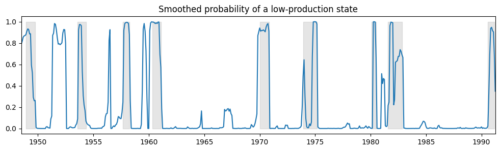
以下に、経済が低生産状態で運営されている確率の平滑化したプロットを示し、比較のために再度NBERの景気後退期間を含めています。

[12]:

fig, ax = plt.subplots(figsize=(12, 3))

ax.plot(res_filardo.smoothed_marginal_probabilities[0])
ax.fill_between(usrec.index, 0, 1, where=usrec["USREC"].values, color="gray", alpha=0.2)
ax.set_xlim(dta_filardo.index[6], dta_filardo.index[-1])
ax.set(title="Smoothed probability of a low-production state")

[12]:

[Text(0.5, 1.0, 'Smoothed probability of a low-production state')]

../../../_images/examples_notebooks_generated_markov_autoregression_22_1.png

時間変動する遷移確率を使用することで、低生産状態の期待される持続期間が時間とともにどのように変化するかを確認できます。

[13]:

res_filardo.expected_durations[0].plot(
    title="Expected duration of a low-production state", figsize=(12, 3)
)

[13]:

<Axes: title={'center': 'Expected duration of a low-production state'}>

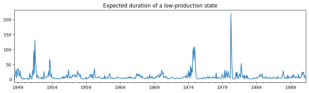
../../../_images/examples_notebooks_generated_markov_autoregression_24_1.png

景気後退時には、低生産状態が続く期間の予想は景気拡大時よりもはるかに長いです。

[ ]:

[ ]:

[ ]:

[ ]:

最終更新日: 2025年01月28日