マルコフスイッチング動的回帰モデル¶

このノートブックは、レジームの変化を伴う動的回帰モデルを推定するために、statsmodels のマルコフスイッチングモデルを使用する例を提供します。これは、Stataのマルコフスイッチングに関するドキュメントの例に従っており、ドキュメントは以下のリンクで確認できます：http://www.stata.com/manuals14/tsmswitch.pdf。

[1]:

%matplotlib inline

import numpy as np
import pandas as pd
import statsmodels.api as sm
import matplotlib.pyplot as plt

# NBER recessions
from pandas_datareader.data import DataReader
from datetime import datetime

usrec = DataReader(
    "USREC", "fred", start=datetime(1947, 1, 1), end=datetime(2013, 4, 1)
)

変動切片を持つ米国政策金利¶

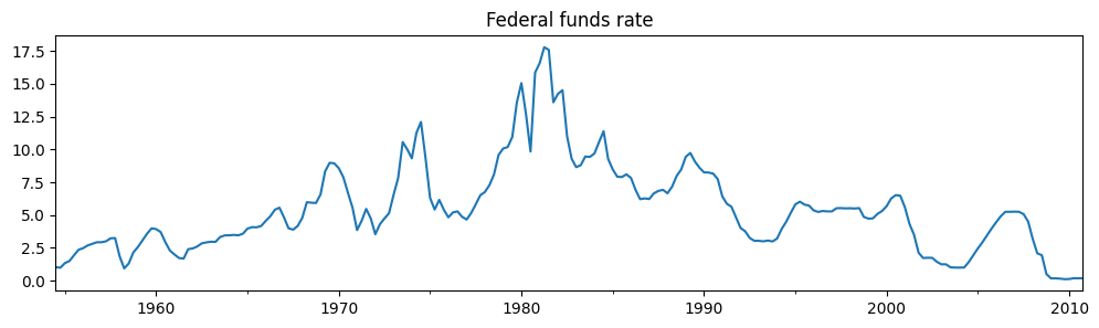
最初の例では、米国政策金利を一定の切片周りのノイズとしてモデル化しますが、この切片は異なるレジーム（状態）で変化します。モデルは単純に次のようになります：

\[r_t = \mu_{S_t} + \varepsilon_t \qquad \varepsilon_t \sim N(0, \sigma^2)\]

ここで、\(S_t \in \{0, 1\}\) はレジームであり、レジーム遷移は次のように記述されます：

\[\begin{split} P(S_t = s_t | S_{t-1} = s_{t-1}) = \begin{bmatrix} p_{00} & p_{10} \\ 1 - p_{00} & 1 - p_{10} \end{bmatrix}\end{split}\]

このモデルのパラメータ（\(p_{00}, p_{10}, \mu_0, \mu_1, \sigma^2\)）は最大尤度法で推定します。

この例で使用されるデータは、次のリンクで確認できます：https://www.stata-press.com/data/r14/usmacro

（翻訳者注：　上記のリンクは切れています。以下のURLに当該のデータファイルと思われるusmacro.dtaが掲載されています。 dtaファイルはpandasのread_stata()関数を用いて直接データフレーム化できます。 https://www.stata-press.com/data/r14/tsmain.html ）

[2]:

# Get the federal funds rate data
from statsmodels.tsa.regime_switching.tests.test_markov_regression import fedfunds

dta_fedfunds = pd.Series(
    fedfunds, index=pd.date_range("1954-07-01", "2010-10-01", freq="QS")
)

# Plot the data
dta_fedfunds.plot(title="Federal funds rate", figsize=(12, 3))

# Fit the model
# (a switching mean is the default of the MarkovRegession model)
mod_fedfunds = sm.tsa.MarkovRegression(dta_fedfunds, k_regimes=2)
res_fedfunds = mod_fedfunds.fit()

../../../_images/examples_notebooks_generated_markov_regression_4_0.png

[3]:

res_fedfunds.summary()

[3]:

Markov Switching Model Results
Dep. Variable:	y	No. Observations:	226
Model:	MarkovRegression	Log Likelihood	-508.636
Date:	Mon, 25 Nov 2024	AIC	1027.272
Time:	13:55:57	BIC	1044.375
Sample:	07-01-1954	HQIC	1034.174
	- 10-01-2010
Covariance Type:	approx

Regime 0 parameters
	coef	std err	z	P>\|z\|	[0.025	0.975]
const	3.7088	0.177	20.988	0.000	3.362	4.055

Regime 1 parameters
	coef	std err	z	P>\|z\|	[0.025	0.975]
const	9.5568	0.300	31.857	0.000	8.969	10.145

Non-switching parameters
	coef	std err	z	P>\|z\|	[0.025	0.975]
sigma2	4.4418	0.425	10.447	0.000	3.608	5.275

Regime transition parameters
	coef	std err	z	P>\|z\|	[0.025	0.975]
p[0->0]	0.9821	0.010	94.443	0.000	0.962	1.002
p[1->0]	0.0504	0.027	1.876	0.061	-0.002	0.103

Warnings:
[1] Covariance matrix calculated using numerical (complex-step) differentiation.

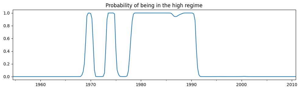
概要の出力から、最初のレジーム（「低金利レジーム」）における米国政策金利の平均値は3.7ドルであり、「高金利レジーム」では9.6ドルであると推定されています。以下に、高金利レジームにいる確率の平滑化したグラフを示します。モデルは、1980年代が高い米国政策金利が存在した時期であったことを示唆しています。

[4]:

res_fedfunds.smoothed_marginal_probabilities[1].plot(
    title="Probability of being in the high regime", figsize=(12, 3)
)

[4]:

<Axes: title={'center': 'Probability of being in the high regime'}>

../../../_images/examples_notebooks_generated_markov_regression_7_1.png

推定された遷移行列から、低水準状態と高水準状態の期待される滞留期間を計算することができます。

[5]:

print(res_fedfunds.expected_durations)

[55.85400626 19.85506546]

低水準の状態は約14年間続くと予想されている一方で、高水準の状態は約5年間しか続かないと予想されています。

変動切片と遅延従属変数を持つ米国政策金利¶

2番目の例では、前のモデルを拡張し、米国政策金利の遅延値を含めています。

\[r_t = \mu_{S_t} + r_{t-1} \beta_{S_t} + \varepsilon_t \qquad \varepsilon_t \sim N(0, \sigma^2)\]

ここで、\(S_t \in \{0, 1\}\) であり、レジームの遷移は次のように表されます。

\[\begin{split} P(S_t = s_t | S_{t-1} = s_{t-1}) = \begin{bmatrix} p_{00} & p_{10} \\ 1 - p_{00} & 1 - p_{10} \end{bmatrix}\end{split}\]

このモデルのパラメータ\(p_{00}, p_{10}, \mu_0, \mu_1, \beta_0, \beta_1, \sigma^2\)を最尤推定法で推定します。

[6]:

# Fit the model
mod_fedfunds2 = sm.tsa.MarkovRegression(
    dta_fedfunds.iloc[1:], k_regimes=2, exog=dta_fedfunds.iloc[:-1]
)
res_fedfunds2 = mod_fedfunds2.fit()

[7]:

res_fedfunds2.summary()

[7]:

Markov Switching Model Results
Dep. Variable:	y	No. Observations:	225
Model:	MarkovRegression	Log Likelihood	-264.711
Date:	Mon, 25 Nov 2024	AIC	543.421
Time:	13:56:03	BIC	567.334
Sample:	10-01-1954	HQIC	553.073
	- 10-01-2010
Covariance Type:	approx

Regime 0 parameters
	coef	std err	z	P>\|z\|	[0.025	0.975]
const	0.7245	0.289	2.510	0.012	0.159	1.290
x1	0.7631	0.034	22.629	0.000	0.697	0.829

Regime 1 parameters
	coef	std err	z	P>\|z\|	[0.025	0.975]
const	-0.0989	0.118	-0.835	0.404	-0.331	0.133
x1	1.0612	0.019	57.351	0.000	1.025	1.097

Non-switching parameters
	coef	std err	z	P>\|z\|	[0.025	0.975]
sigma2	0.4783	0.050	9.642	0.000	0.381	0.576

Regime transition parameters
	coef	std err	z	P>\|z\|	[0.025	0.975]
p[0->0]	0.6378	0.120	5.304	0.000	0.402	0.874
p[1->0]	0.1306	0.050	2.634	0.008	0.033	0.228

Warnings:
[1] Covariance matrix calculated using numerical (complex-step) differentiation.

要約結果から注目すべき点がいくつかあります：

情報量基準が大幅に減少しており、これはこのモデルが前のモデルよりも適合度が良いことを示しています。
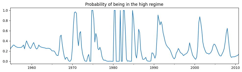
切片に関して、状態の解釈が入れ替わっています。現在、最初の状態は高い切片を持ち、2番目の状態は低い切片を持っています。

高い状態の平滑化された確率を調べると、現在ではかなりの変動が見られます。

[8]:

res_fedfunds2.smoothed_marginal_probabilities[0].plot(
    title="Probability of being in the high regime", figsize=(12, 3)
)

[8]:

<Axes: title={'center': 'Probability of being in the high regime'}>

../../../_images/examples_notebooks_generated_markov_regression_15_1.png

最後に、各レジームの予想される期間はかなり短くなりました。

[9]:

print(res_fedfunds2.expected_durations)

[2.76105188 7.65529154]

2つまたは3つのレジームを持つテイラー・ルール¶

現在、出力ギャップの指標とインフレの指標という2つの追加的な外生変数を含め、データに適したモデルを確認するために、2レジームおよび3レジームの切替型テイラー・ルールを推定します。

モデルの推定はしばしば難しいため、3レジームモデルでは、結果を改善するために開始パラメータの探索を行い、20回のランダム検索を指定して実行します。

[10]:

# Get the additional data
from statsmodels.tsa.regime_switching.tests.test_markov_regression import ogap, inf

dta_ogap = pd.Series(ogap, index=pd.date_range("1954-07-01", "2010-10-01", freq="QS"))
dta_inf = pd.Series(inf, index=pd.date_range("1954-07-01", "2010-10-01", freq="QS"))

exog = pd.concat((dta_fedfunds.shift(), dta_ogap, dta_inf), axis=1).iloc[4:]

# Fit the 2-regime model
mod_fedfunds3 = sm.tsa.MarkovRegression(dta_fedfunds.iloc[4:], k_regimes=2, exog=exog)
res_fedfunds3 = mod_fedfunds3.fit()

# Fit the 3-regime model
np.random.seed(12345)
mod_fedfunds4 = sm.tsa.MarkovRegression(dta_fedfunds.iloc[4:], k_regimes=3, exog=exog)
res_fedfunds4 = mod_fedfunds4.fit(search_reps=20)

[11]:

res_fedfunds3.summary()

[11]:

Markov Switching Model Results
Dep. Variable:	y	No. Observations:	222
Model:	MarkovRegression	Log Likelihood	-229.256
Date:	Mon, 25 Nov 2024	AIC	480.512
Time:	13:56:09	BIC	517.942
Sample:	07-01-1955	HQIC	495.624
	- 10-01-2010
Covariance Type:	approx

Regime 0 parameters
	coef	std err	z	P>\|z\|	[0.025	0.975]
const	0.6555	0.137	4.771	0.000	0.386	0.925
x1	0.8314	0.033	24.951	0.000	0.766	0.897
x2	0.1355	0.029	4.609	0.000	0.078	0.193
x3	-0.0274	0.041	-0.671	0.502	-0.107	0.053

Regime 1 parameters
	coef	std err	z	P>\|z\|	[0.025	0.975]
const	-0.0945	0.128	-0.739	0.460	-0.345	0.156
x1	0.9293	0.027	34.309	0.000	0.876	0.982
x2	0.0343	0.024	1.429	0.153	-0.013	0.081
x3	0.2125	0.030	7.147	0.000	0.154	0.271

Non-switching parameters
	coef	std err	z	P>\|z\|	[0.025	0.975]
sigma2	0.3323	0.035	9.526	0.000	0.264	0.401

Regime transition parameters
	coef	std err	z	P>\|z\|	[0.025	0.975]
p[0->0]	0.7279	0.093	7.828	0.000	0.546	0.910
p[1->0]	0.2115	0.064	3.298	0.001	0.086	0.337

Warnings:
[1] Covariance matrix calculated using numerical (complex-step) differentiation.

[12]:

res_fedfunds4.summary()

[12]:

Markov Switching Model Results
Dep. Variable:	y	No. Observations:	222
Model:	MarkovRegression	Log Likelihood	-180.806
Date:	Mon, 25 Nov 2024	AIC	399.611
Time:	13:56:09	BIC	464.262
Sample:	07-01-1955	HQIC	425.713
	- 10-01-2010
Covariance Type:	approx

Regime 0 parameters
	coef	std err	z	P>\|z\|	[0.025	0.975]
const	-1.0250	0.290	-3.531	0.000	-1.594	-0.456
x1	0.3277	0.086	3.812	0.000	0.159	0.496
x2	0.2036	0.049	4.152	0.000	0.107	0.300
x3	1.1381	0.081	13.977	0.000	0.978	1.298

Regime 1 parameters
	coef	std err	z	P>\|z\|	[0.025	0.975]
const	-0.0259	0.087	-0.298	0.765	-0.196	0.144
x1	0.9737	0.019	50.265	0.000	0.936	1.012
x2	0.0341	0.017	2.030	0.042	0.001	0.067
x3	0.1215	0.022	5.606	0.000	0.079	0.164

Regime 2 parameters
	coef	std err	z	P>\|z\|	[0.025	0.975]
const	0.7346	0.130	5.632	0.000	0.479	0.990
x1	0.8436	0.024	35.198	0.000	0.797	0.891
x2	0.1633	0.025	6.515	0.000	0.114	0.212
x3	-0.0499	0.027	-1.835	0.067	-0.103	0.003

Non-switching parameters
	coef	std err	z	P>\|z\|	[0.025	0.975]
sigma2	0.1660	0.018	9.240	0.000	0.131	0.201

Regime transition parameters
	coef	std err	z	P>\|z\|	[0.025	0.975]
p[0->0]	0.7214	0.117	6.177	0.000	0.493	0.950
p[1->0]	4.001e-08	nan	nan	nan	nan	nan
p[2->0]	0.0783	0.038	2.079	0.038	0.004	0.152
p[0->1]	0.1044	0.095	1.103	0.270	-0.081	0.290
p[1->1]	0.8259	0.054	15.208	0.000	0.719	0.932
p[2->1]	0.2288	0.073	3.150	0.002	0.086	0.371

Warnings:
[1] Covariance matrix calculated using numerical (complex-step) differentiation.

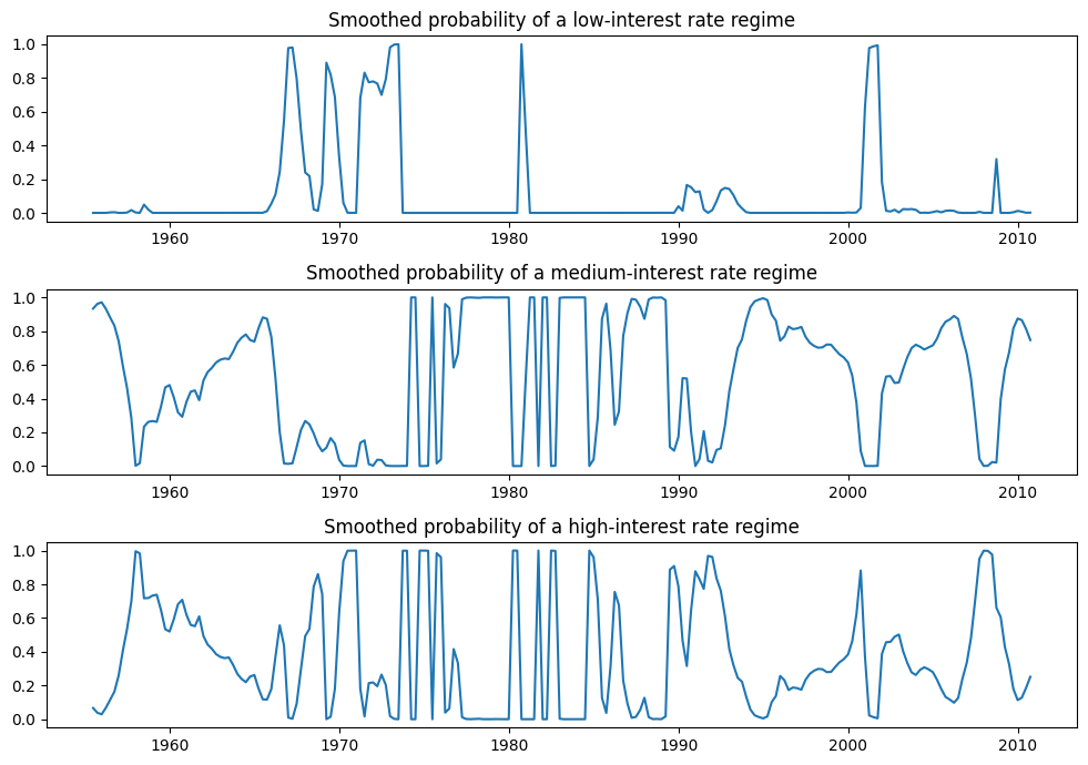
情報量基準が低いため、低金利・中金利・高金利のレジームを解釈した3状態モデルを選好するかもしれません。各レジームの平滑化された確率は以下にプロットされています。

[13]:

fig, axes = plt.subplots(3, figsize=(10, 7))

ax = axes[0]
ax.plot(res_fedfunds4.smoothed_marginal_probabilities[0])
ax.set(title="Smoothed probability of a low-interest rate regime")

ax = axes[1]
ax.plot(res_fedfunds4.smoothed_marginal_probabilities[1])
ax.set(title="Smoothed probability of a medium-interest rate regime")

ax = axes[2]
ax.plot(res_fedfunds4.smoothed_marginal_probabilities[2])
ax.set(title="Smoothed probability of a high-interest rate regime")

fig.tight_layout()

../../../_images/examples_notebooks_generated_markov_regression_23_0.png

分散の切り替え¶

また、分散の切り替えにも対応できます。特に、次のモデルを考えます。

\[y_t = \mu_{S_t} + y_{t-1} \beta_{S_t} + \varepsilon_t \quad \varepsilon_t \sim N(0, \sigma_{S_t}^2)\]

このモデルのパラメータ \(p_{00}, p_{10}, \mu_0, \mu_1, \beta_0, \beta_1, \sigma_0^2, \sigma_1^2\) を最大尤度法で推定します。

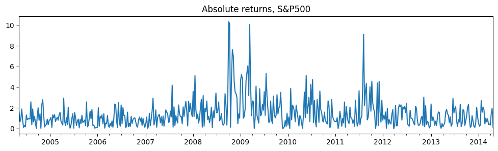
この応用は、株式の絶対リターンに関するもので、データは https://www.stata-press.com/data/r14/snp500 で確認できます。

[14]:

# Get the federal funds rate data
from statsmodels.tsa.regime_switching.tests.test_markov_regression import areturns

dta_areturns = pd.Series(
    areturns, index=pd.date_range("2004-05-04", "2014-5-03", freq="W")
)

# Plot the data
dta_areturns.plot(title="Absolute returns, S&P500", figsize=(12, 3))

# Fit the model
mod_areturns = sm.tsa.MarkovRegression(
    dta_areturns.iloc[1:],
    k_regimes=2,
    exog=dta_areturns.iloc[:-1],
    switching_variance=True,
)
res_areturns = mod_areturns.fit()

../../../_images/examples_notebooks_generated_markov_regression_25_0.png

[15]:

res_areturns.summary()

[15]:

Markov Switching Model Results
Dep. Variable:	y	No. Observations:	520
Model:	MarkovRegression	Log Likelihood	-745.798
Date:	Mon, 25 Nov 2024	AIC	1507.595
Time:	13:56:11	BIC	1541.626
Sample:	05-16-2004	HQIC	1520.926
	- 04-27-2014
Covariance Type:	approx

Regime 0 parameters
	coef	std err	z	P>\|z\|	[0.025	0.975]
const	0.7641	0.078	9.761	0.000	0.611	0.918
x1	0.0791	0.030	2.620	0.009	0.020	0.138
sigma2	0.3476	0.061	5.694	0.000	0.228	0.467

Regime 1 parameters
	coef	std err	z	P>\|z\|	[0.025	0.975]
const	1.9728	0.278	7.086	0.000	1.427	2.518
x1	0.5280	0.086	6.155	0.000	0.360	0.696
sigma2	2.5771	0.405	6.357	0.000	1.783	3.372

Regime transition parameters
	coef	std err	z	P>\|z\|	[0.025	0.975]
p[0->0]	0.7531	0.063	11.871	0.000	0.629	0.877
p[1->0]	0.6825	0.066	10.301	0.000	0.553	0.812

Warnings:
[1] Covariance matrix calculated using numerical (complex-step) differentiation.

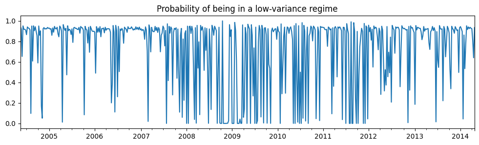
最初のレジームは低分散のレジームで、2番目のレジームは高分散のレジームです。以下に、低分散レジームにいる確率をプロットします。2008年から2012年の間には、どのレジームが経済を支配しているのかは明確な兆候が見られません。

[16]:

res_areturns.smoothed_marginal_probabilities[0].plot(
    title="Probability of being in a low-variance regime", figsize=(12, 3)
)

[16]:

<Axes: title={'center': 'Probability of being in a low-variance regime'}>

../../../_images/examples_notebooks_generated_markov_regression_28_1.png

[ ]:

[ ]:

[ ]:

[ ]:

最終更新日: 2025年01月28日