LOESSを用いた多重季節性-トレンド分解(MSTL)
このノートブックでは、MSTL [1] を使用して、時系列をトレンド成分、複数の季節性成分、および残差成分に分解する方法を示します。MSTLは、STL(LOESSを使用した季節性-トレンド分解)を使用して、時系列から季節性成分を反復的に抽出します。MSTLへの主な入力は次の通りです:
periods- 各季節性成分の周期(例えば、日次および週次の季節性を持つ時系列データの場合、periods=(24, 24*7)となります)。windows- 各周期に対する季節性スムージャーの長さ。これが大きいほど、季節性成分の変動が小さくなります。奇数である必要があります。Noneの場合、元の論文[1]で実験によって決定されたデフォルト値が使用されます。lmbda- 分解前に行うBox-Cox変換のλパラメータ。Noneの場合は変換は行われません。"auto"の場合、データから自動的に適切なλの値が選択されます。iterate- 季節性成分を洗練させるために使用する反復回数。stl_kwargs- STLに渡すことができる他のパラメータ(例:robust、seasonal_degなど)。詳細はSTLドキュメントを参照してください。
この実装には1といくつかの重要な違いがあります。欠損データはMSTLクラスの外部で処理する必要があります。論文で提案されたアルゴリズムは、季節性がない場合を処理しますが、この実装では少なくとも1つの季節性成分があると仮定しています。
まず、必要なパッケージをインポートし、グラフィック環境を準備し、データを準備します。
[1]:
import matplotlib.pyplot as plt
import datetime
import pandas as pd
import numpy as np
import seaborn as sns
from pandas.plotting import register_matplotlib_converters

from statsmodels.tsa.seasonal import MSTL
from statsmodels.tsa.seasonal import DecomposeResult

register_matplotlib_converters()
sns.set_style("darkgrid")
[2]:
plt.rc("figure", figsize=(16, 12))
plt.rc("font", size=13)
MSTLを玩具的なデータセットに適用した例
複数の季節性を持つ玩具的なデータセットを作成する
我々は、日次および週次の季節性を持ち、サイン波に従う時系列を時間単位の頻度で作成します。ノートブックの後半で、より現実的な例を示します。
[3]:
t = np.arange(1, 1000)
daily_seasonality = 5 * np.sin(2 * np.pi * t / 24)
weekly_seasonality = 10 * np.sin(2 * np.pi * t / (24 * 7))
trend = 0.0001 * t**2
y = trend + daily_seasonality + weekly_seasonality + np.random.randn(len(t))
ts = pd.date_range(start="2020-01-01", freq="H", periods=len(t))
df = pd.DataFrame(data=y, index=ts, columns=["y"])
[4]:
df.head()
[4]:
| y | |
|---|---|
| 2020-01-01 00:00:00 | 1.572177 |
| 2020-01-01 01:00:00 | 2.438489 |
| 2020-01-01 02:00:00 | 4.791373 |
| 2020-01-01 03:00:00 | 7.587587 |
| 2020-01-01 04:00:00 | 6.458602 |
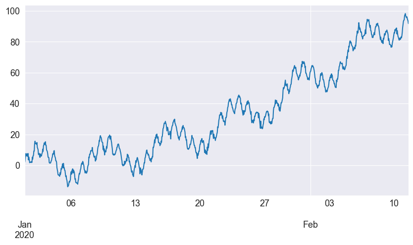
時系列をプロットしましょう。
[5]:
df["y"].plot(figsize=[10, 5])
[5]:
<Axes: >
MSTLを使って玩具的なデータセットを分解する
時系列をトレンド成分、日次および週次の季節成分、残差成分に分解するためにMSTLを使用しましょう。
[6]:
mstl = MSTL(df["y"], periods=[24, 24 * 7])
res = mstl.fit()
入力がpandasのデータフレームの場合、季節成分の出力もデータフレームになります。各成分の期間は列名に反映されます。
[7]:
res.seasonal.head()
[7]:
| seasonal_24 | seasonal_168 | |
|---|---|---|
| 2020-01-01 00:00:00 | 0.196574 | 1.355488 |
| 2020-01-01 01:00:00 | 1.643201 | 1.357137 |
| 2020-01-01 02:00:00 | 3.760683 | 1.772219 |
| 2020-01-01 03:00:00 | 6.255390 | 1.066101 |
| 2020-01-01 04:00:00 | 4.387905 | 2.504967 |
[8]:
ax = res.plot()
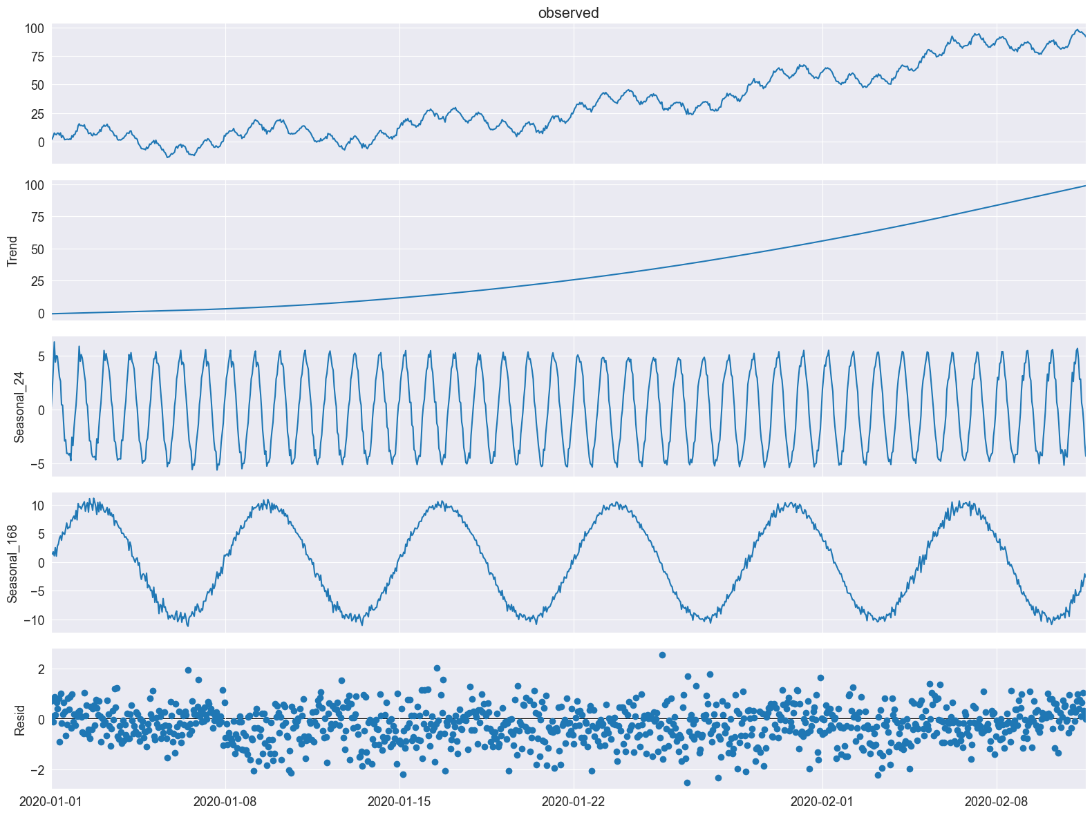
時間単位および週単位の季節成分が抽出されたことが分かります。
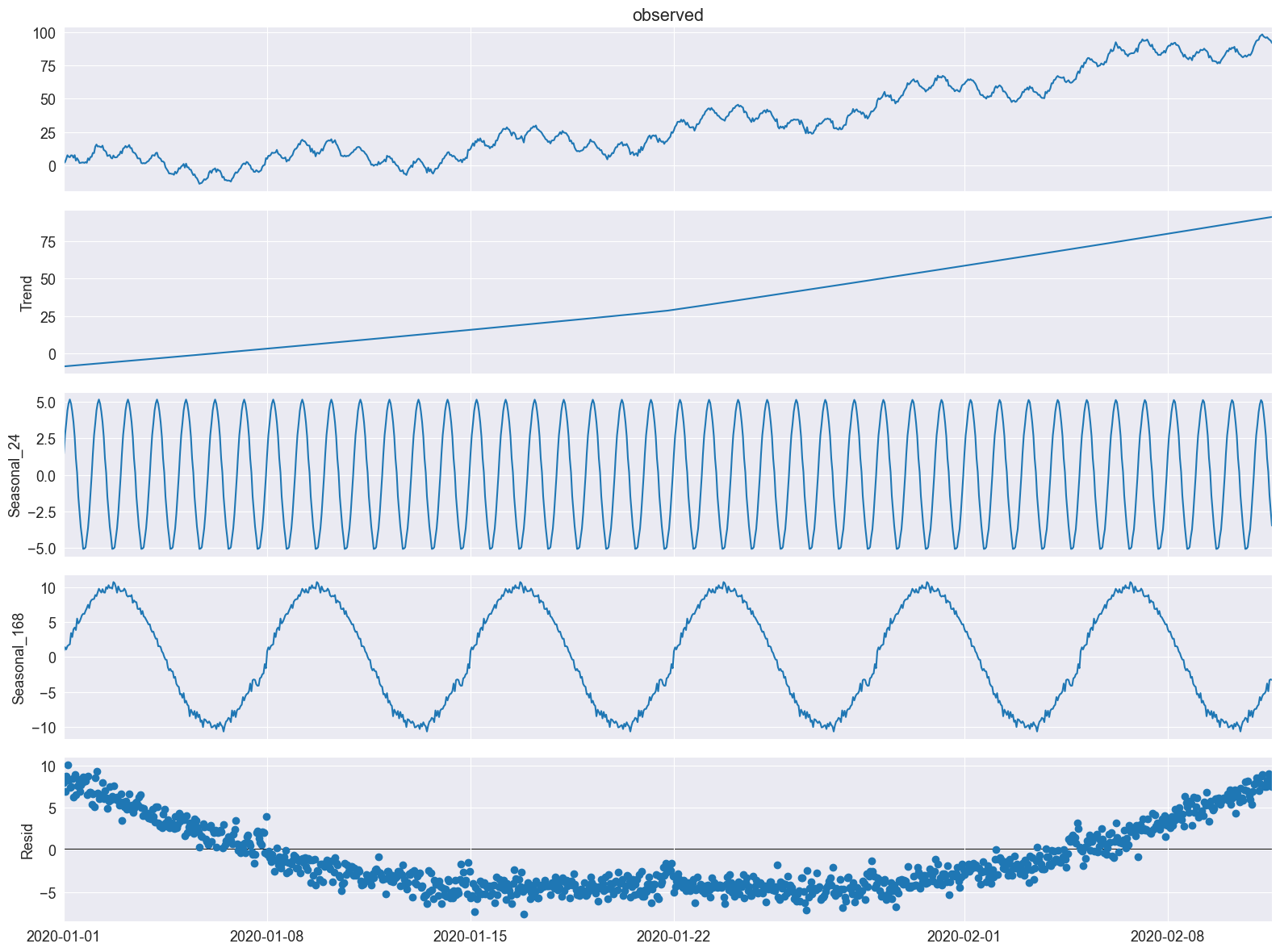
period と seasonal 以外のSTLパラメータ(これらは MSTL では periods と windows によって設定されます)は、stl_kwargs に辞書形式で arg:value のペアを渡すことによって設定できます(これを今から例で示します)。
ここでは、STLのトレンドスムーザーを trend で、季節調整の多項式の次数を seasonal_deg で設定できることを示します。また、windows、seasonal_deg、iterate のパラメータも明示的に設定します。最適なフィットにはならないかもしれませんが、これは MSTL クラスにこれらのパラメータを渡す方法の一例です。
[9]:
mstl = MSTL(
    df,
    periods=[24, 24 * 7],  # The periods and windows must be the same length and will correspond to one another.
    windows=[101, 101],  # Setting this large along with `seasonal_deg=0` will force the seasonality to be periodic.
    iterate=3,
    stl_kwargs={
                "trend":1001, # Setting this large will force the trend to be smoother.
                "seasonal_deg":0, # Means the seasonal smoother is fit with a moving average.
               }
)
res = mstl.fit()
ax = res.plot()
MSTLを電力需要データセットに適用
データを準備する
[10]:
url = "https://raw.githubusercontent.com/tidyverts/tsibbledata/master/data-raw/vic_elec/VIC2015/demand.csv"
df = pd.read_csv(url)
[11]:
df.head()
[11]:
| Date | Period | OperationalLessIndustrial | Industrial | |
|---|---|---|---|---|
| 0 | 37257 | 1 | 3535.867064 | 1086.132936 |
| 1 | 37257 | 2 | 3383.499028 | 1088.500972 |
| 2 | 37257 | 3 | 3655.527552 | 1084.472448 |
| 3 | 37257 | 4 | 3510.446636 | 1085.553364 |
| 4 | 37257 | 5 | 3294.697156 | 1081.302844 |
日付は、基準日からの日数を表す整数値です。このデータセットの基準日はこちらおよびこちらから確認でき、「1899-12-30」となっています。Periodの整数値は1日の30分間隔を表しており、1日につき48の区分があります。
日付と日時を抽出してみましょう。
[12]:
df["Date"] = df["Date"].apply(lambda x: pd.Timestamp("1899-12-30") + pd.Timedelta(x, unit="days"))
df["ds"] = df["Date"] + pd.to_timedelta((df["Period"]-1)*30, unit="m")
私たちは「OperationalLessIndustrial」に注目します。これは、特定の高エネルギー産業ユーザーによる需要を除いた電力需要を表しています。このデータを1時間単位にリサンプリングし、元のMSTL論文 [1]と同じ期間、つまり2012年の最初の149日間にデータをフィルタリングします。
[13]:
timeseries = df[["ds", "OperationalLessIndustrial"]]
timeseries.columns = ["ds", "y"] # Rename to OperationalLessIndustrial to y for simplicity.

# Filter for first 149 days of 2012.
start_date = pd.to_datetime("2012-01-01")
end_date = start_date + pd.Timedelta("149D")
mask = (timeseries["ds"] >= start_date) & (timeseries["ds"] < end_date)
timeseries = timeseries[mask]

# Resample to hourly
timeseries = timeseries.set_index("ds").resample("H").sum()
timeseries.head()
[13]:
| y | |
|---|---|
| ds | |
| 2012-01-01 00:00:00 | 7926.529376 |
| 2012-01-01 01:00:00 | 7901.826990 |
| 2012-01-01 02:00:00 | 7255.721350 |
| 2012-01-01 03:00:00 | 6792.503352 |
| 2012-01-01 04:00:00 | 6635.984460 |
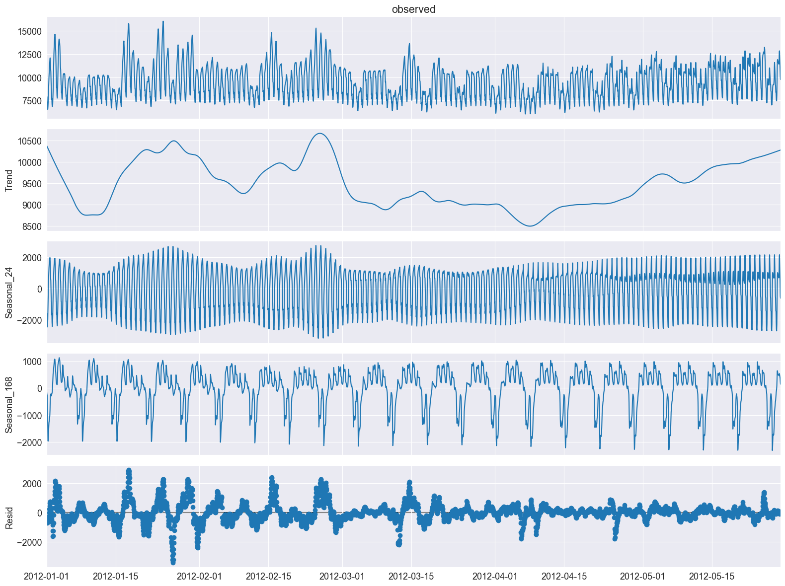
MSTLを使用した電力需要の分解
このデータセットにMSTLを適用してみましょう。
注: stl_kwargsは、[1]で示された結果に近いものを得るために設定されています。この論文ではRを使用しており、そのため基礎となるSTLパラメータのデフォルト設定が若干異なります。実際には、inner_iterやouter_iterを明示的に手動設定することはまれです。
[14]:
mstl = MSTL(timeseries["y"], periods=[24, 24 * 7], iterate=3, stl_kwargs={"seasonal_deg": 0,
                                                                          "inner_iter": 2,
                                                                          "outer_iter": 0})
res = mstl.fit() # Use .fit() to perform and return the decomposition
ax = res.plot()
plt.tight_layout()
複数の季節成分は、seasonal属性にpandasデータフレームとして格納されています。
[15]:
res.seasonal.head()
[15]:
| seasonal_24 | seasonal_168 | |
|---|---|---|
| ds | ||
| 2012-01-01 00:00:00 | -1685.986297 | -161.807086 |
| 2012-01-01 01:00:00 | -1591.640845 | -229.788887 |
| 2012-01-01 02:00:00 | -2192.989492 | -260.121300 |
| 2012-01-01 03:00:00 | -2442.169359 | -388.484499 |
| 2012-01-01 04:00:00 | -2357.492551 | -660.245476 |
季節性の要素をもう少し詳しく調べ、最初の数日間や数週間を見て、日次および週次の季節性を確認してみましょう。
[16]:
fig, ax = plt.subplots(nrows=2, figsize=[10,10])
res.seasonal["seasonal_24"].iloc[:24*3].plot(ax=ax[0])
ax[0].set_ylabel("seasonal_24")
ax[0].set_title("Daily seasonality")

res.seasonal["seasonal_168"].iloc[:24*7*3].plot(ax=ax[1])
ax[1].set_ylabel("seasonal_168")
ax[1].set_title("Weekly seasonality")

plt.tight_layout()
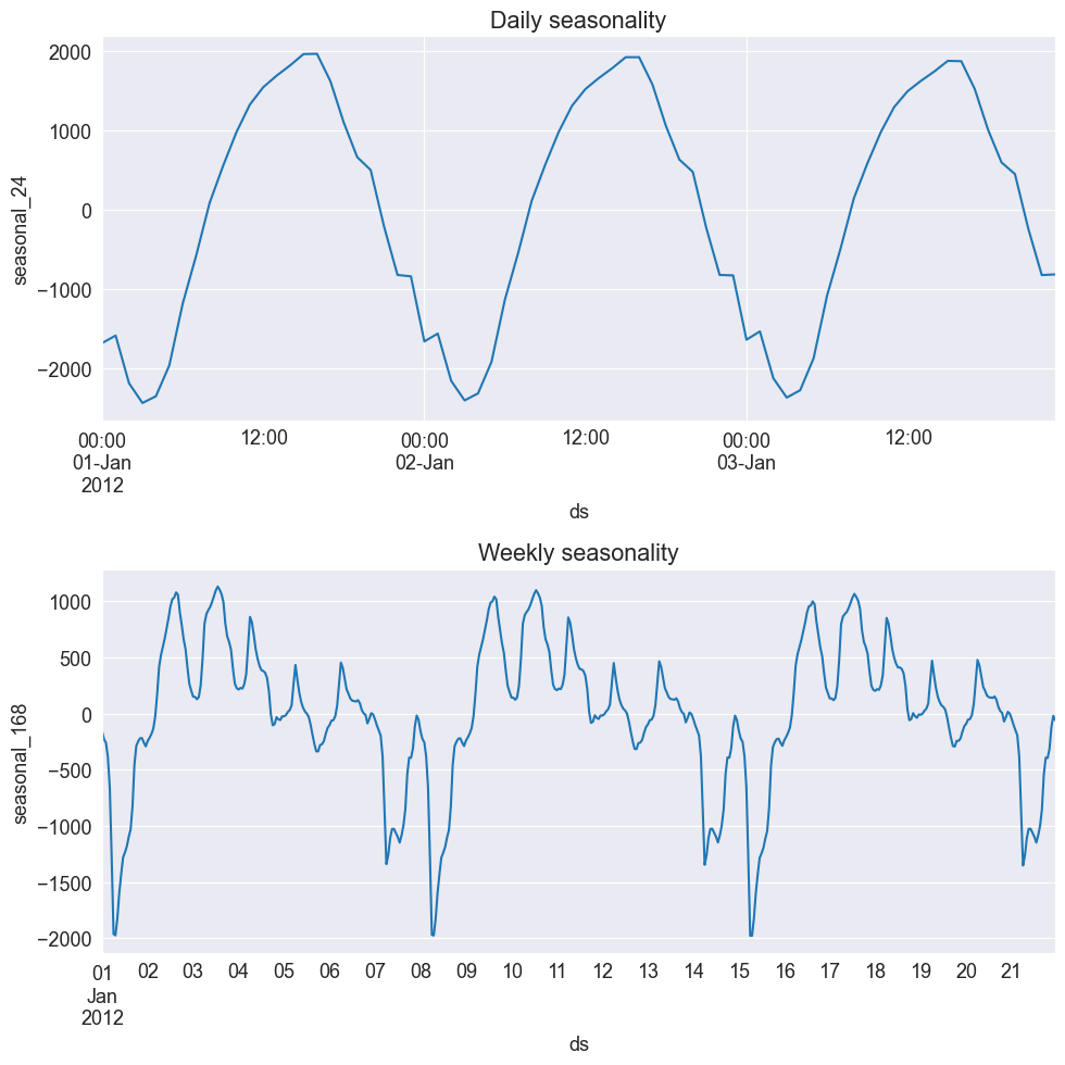
電力需要の日次季節性が十分に捉えられていることがわかります。これは1月の最初の数日を示しており、オーストラリアでは夏の時期にあたるため、エアコンの使用が原因で午後に需要がピークになると考えられます。
週次季節性については、週末に使用量が減少することが確認できます。
MSTLの利点の1つは、時間の経過とともに変化する季節性を捉えることができる点です。それでは、5月の涼しい月の季節性を見てみましょう。
[17]:
fig, ax = plt.subplots(nrows=2, figsize=[10,10])
mask = res.seasonal.index.month==5
res.seasonal[mask]["seasonal_24"].iloc[:24*3].plot(ax=ax[0])
ax[0].set_ylabel("seasonal_24")
ax[0].set_title("Daily seasonality")

res.seasonal[mask]["seasonal_168"].iloc[:24*7*3].plot(ax=ax[1])
ax[1].set_ylabel("seasonal_168")
ax[1].set_title("Weekly seasonality")

plt.tight_layout()
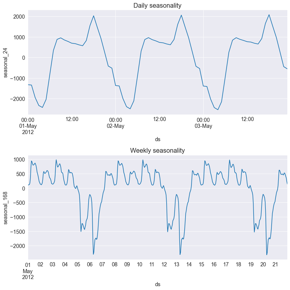
これで、夕方に新たなピークがあることがわかります! これは、夕方に必要となる暖房や照明に関連している可能性があります。そのため、これは納得のいく現象です。また、週末に需要が低下する主な週ごとのパターンが引き続き見られることも確認できます。
他のコンポーネントは、trend と resid 属性からも抽出できます。
[18]:
display(res.trend.head()) # trend component
display(res.resid.head()) # residual component
ds
2012-01-01 00:00:00    10373.942662
2012-01-01 01:00:00    10363.488489
2012-01-01 02:00:00    10353.037721
2012-01-01 03:00:00    10342.590527
2012-01-01 04:00:00    10332.147100
Freq: H, Name: trend, dtype: float64
ds
2012-01-01 00:00:00   -599.619903
2012-01-01 01:00:00   -640.231767
2012-01-01 02:00:00   -644.205579
2012-01-01 03:00:00   -719.433316
2012-01-01 04:00:00   -678.424613
Freq: H, Name: resid, dtype: float64
これで終わりです!MSTLを使用すれば、複数の季節性を持つ時系列データの分解を行うことができます!