指数平滑法¶

HyndmanとAthanasopoulosによる優れた専門書「指数平滑法」に関する第7章を取り上げます【1】。章の中で紹介されているすべての例を順を追って進めていきます。

【1】 Hyndman, Rob J., and George Athanasopoulos. Forecasting: principles and practice. OTexts, 2014.

データの読み込み¶

まず、データを読み込みます。便宜上、ノートブックにRデータを含めています。

[1]:

import os
import numpy as np
import pandas as pd
import matplotlib.pyplot as plt
from statsmodels.tsa.api import ExponentialSmoothing, SimpleExpSmoothing, Holt

%matplotlib inline

data = [
6565,
4733,
663,
6322,
2713,
5881,
3325,
1494,
0482,
792,
2689,
211,
]
index = pd.date_range(start="1996", end="2008", freq="A")
oildata = pd.Series(data, index)

data = [
5534,
86,
8866,
9293,
8885,
8314,
0751,
9535,
1857,
5797,
5776,
4774,
0216,
3864,
5966,
]
index = pd.date_range(start="1990", end="2005", freq="A")
air = pd.Series(data, index)

data = [
9177,
3072,
6626,
6394,
5158,
834,
309,
4742,
8307,
2867,
3311,
3724,
884,
2441,
6006,
2554,
4597,
4138,
7893,
3852,
2979,
3705,
5629,
1236,
7495,
2339,
9468,
6971,
4993,
2705,
2428,
]
index = pd.date_range(start="1970", end="2001", freq="A")
livestock2 = pd.Series(data, index)

data = [407.9979, 403.4608, 413.8249, 428.105, 445.3387, 452.9942, 455.7402]
index = pd.date_range(start="2001", end="2008", freq="A")
livestock3 = pd.Series(data, index)

data = [
7275,
0418,
3281,
3287,
2132,
3463,
4829,
9777,
9015,
1802,
7179,
4202,
2069,
8872,
9783,
7725,
5586,
8509,
0764,
6423,
7668,
1919,
3197,
9137,
]
index = pd.date_range(start="2005", end="2010-Q4", freq="QS-OCT")
aust = pd.Series(data, index)

C:\Users\user\AppData\Local\Temp\ipykernel_10924\327638849.py:23: FutureWarning: 'A' is deprecated and will be removed in a future version, please use 'YE' instead.
  index = pd.date_range(start="1996", end="2008", freq="A")
C:\Users\user\AppData\Local\Temp\ipykernel_10924\327638849.py:43: FutureWarning: 'A' is deprecated and will be removed in a future version, please use 'YE' instead.
  index = pd.date_range(start="1990", end="2005", freq="A")
C:\Users\user\AppData\Local\Temp\ipykernel_10924\327638849.py:79: FutureWarning: 'A' is deprecated and will be removed in a future version, please use 'YE' instead.
  index = pd.date_range(start="1970", end="2001", freq="A")
C:\Users\user\AppData\Local\Temp\ipykernel_10924\327638849.py:83: FutureWarning: 'A' is deprecated and will be removed in a future version, please use 'YE' instead.
  index = pd.date_range(start="2001", end="2008", freq="A")

単純指数平滑法¶

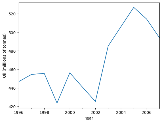
以下の石油データを予測するために、単純指数平滑法を使用しましょう。

[2]:

ax = oildata.plot()
ax.set_xlabel("Year")
ax.set_ylabel("Oil (millions of tonnes)")
print("Figure 7.1: Oil production in Saudi Arabia from 1996 to 2007.")

Figure 7.1: Oil production in Saudi Arabia from 1996 to 2007.

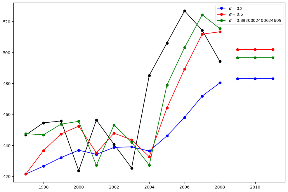
../../../_images/examples_notebooks_generated_exponential_smoothing_4_1.png

ここでは、単純指数平滑法の3つのバリアントを実行します：

fit1では、自己最適化を使用せず、代わりにモデルに明示的に$\alpha=0.2$のパラメータを提供します。
fit2では、上記のように$\alpha=0.6$を選択します。
fit3では、statsmodelsに自動的に最適化された$\alpha$値を見つけさせます。これが推奨されるアプローチです。

[3]:

fit1 = SimpleExpSmoothing(oildata, initialization_method="heuristic").fit(
    smoothing_level=0.2, optimized=False
)
fcast1 = fit1.forecast(3).rename(r"$\alpha=0.2$")
fit2 = SimpleExpSmoothing(oildata, initialization_method="heuristic").fit(
    smoothing_level=0.6, optimized=False
)
fcast2 = fit2.forecast(3).rename(r"$\alpha=0.6$")
fit3 = SimpleExpSmoothing(oildata, initialization_method="estimated").fit()
fcast3 = fit3.forecast(3).rename(r"$\alpha=%s$" % fit3.model.params["smoothing_level"])

plt.figure(figsize=(12, 8))
plt.plot(oildata, marker="o", color="black")
plt.plot(fit1.fittedvalues, marker="o", color="blue")
(line1,) = plt.plot(fcast1, marker="o", color="blue")
plt.plot(fit2.fittedvalues, marker="o", color="red")
(line2,) = plt.plot(fcast2, marker="o", color="red")
plt.plot(fit3.fittedvalues, marker="o", color="green")
(line3,) = plt.plot(fcast3, marker="o", color="green")
plt.legend([line1, line2, line3], [fcast1.name, fcast2.name, fcast3.name])

[3]:

<matplotlib.legend.Legend at 0x2a651ac68f0>

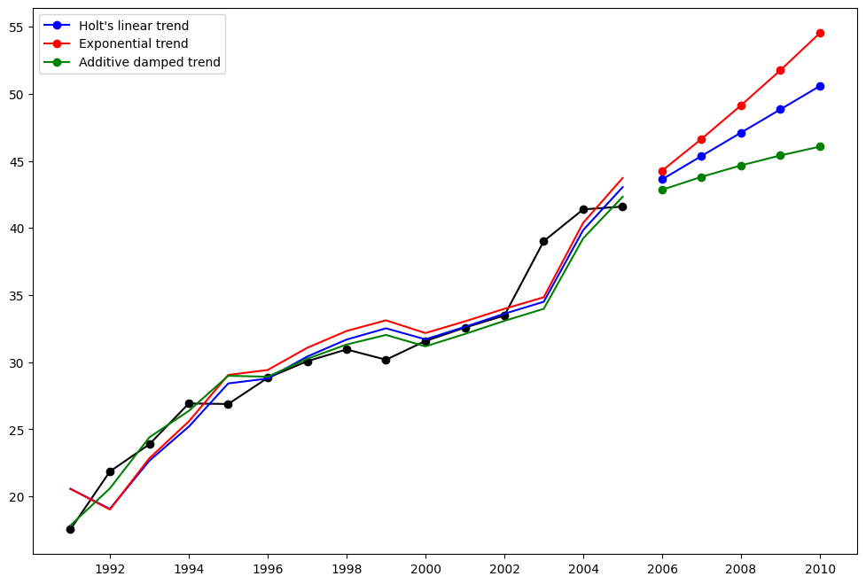
../../../_images/examples_notebooks_generated_exponential_smoothing_6_1.png

ホルト法¶

別の例を見てみましょう。今回は大気汚染データを使用し、ホルト法を適用します。再び3つの例を適合させます。

fit1 では、最適化器を使用せず、$\alpha=0.8$ と $\beta=0.2$ の明示的な値を提供します。
fit2 では、fit1 と同様に行いますが、ホルトの加法モデルではなく指数モデルを使用します。
fit3 では、ホルトの加法モデルの減衰版を使用し、減衰パラメータ$\phi$を最適化可能にし、$\alpha=0.8$ と $\beta=0.2$ の値は固定します。

[4]:

fit1 = Holt(air, initialization_method="estimated").fit(
    smoothing_level=0.8, smoothing_trend=0.2, optimized=False
)
fcast1 = fit1.forecast(5).rename("Holt's linear trend")
fit2 = Holt(air, exponential=True, initialization_method="estimated").fit(
    smoothing_level=0.8, smoothing_trend=0.2, optimized=False
)
fcast2 = fit2.forecast(5).rename("Exponential trend")
fit3 = Holt(air, damped_trend=True, initialization_method="estimated").fit(
    smoothing_level=0.8, smoothing_trend=0.2
)
fcast3 = fit3.forecast(5).rename("Additive damped trend")

plt.figure(figsize=(12, 8))
plt.plot(air, marker="o", color="black")
plt.plot(fit1.fittedvalues, color="blue")
(line1,) = plt.plot(fcast1, marker="o", color="blue")
plt.plot(fit2.fittedvalues, color="red")
(line2,) = plt.plot(fcast2, marker="o", color="red")
plt.plot(fit3.fittedvalues, color="green")
(line3,) = plt.plot(fcast3, marker="o", color="green")
plt.legend([line1, line2, line3], [fcast1.name, fcast2.name, fcast3.name])

[4]:

<matplotlib.legend.Legend at 0x2a671105a80>

../../../_images/examples_notebooks_generated_exponential_smoothing_8_1.png

季節調整済みデータ¶

季節調整済みの家畜データを見てみましょう。ここでは、5つのホルトモデルを適合させます。

下の表では、指数型と加法型、減衰型と非減衰型を使用した場合の結果を比較できます。

注: fit4はパラメータ$\phi$を最適化できないため、$\phi=0.98$の固定値を提供しています。

[5]:

fit1 = SimpleExpSmoothing(livestock2, initialization_method="estimated").fit()
fit2 = Holt(livestock2, initialization_method="estimated").fit()
fit3 = Holt(livestock2, exponential=True, initialization_method="estimated").fit()
fit4 = Holt(livestock2, damped_trend=True, initialization_method="estimated").fit(
    damping_trend=0.98
)
fit5 = Holt(
    livestock2, exponential=True, damped_trend=True, initialization_method="estimated"
).fit()
params = [
    "smoothing_level",
    "smoothing_trend",
    "damping_trend",
    "initial_level",
    "initial_trend",
]
results = pd.DataFrame(
    index=[r"$\alpha$", r"$\beta$", r"$\phi$", r"$l_0$", "$b_0$", "SSE"],
    columns=["SES", "Holt's", "Exponential", "Additive", "Multiplicative"],
)
results["SES"] = [fit1.params[p] for p in params] + [fit1.sse]
results["Holt's"] = [fit2.params[p] for p in params] + [fit2.sse]
results["Exponential"] = [fit3.params[p] for p in params] + [fit3.sse]
results["Additive"] = [fit4.params[p] for p in params] + [fit4.sse]
results["Multiplicative"] = [fit5.params[p] for p in params] + [fit5.sse]
results

[5]:

	SES	Holt's	Exponential	Additive	Multiplicative
$\alpha$	1.000000	0.974338	0.977642	0.978843	9.749169e-01
$\beta$	NaN	0.000000	0.000000	0.000008	5.952922e-10
$\phi$	NaN	NaN	NaN	0.980000	9.816500e-01
$l_0$	263.917703	258.882683	260.335599	257.357716	2.589521e+02
$b_0$	NaN	5.010856	1.013780	6.645297	1.038139e+00
SSE	6761.350235	6004.138207	6104.194782	6036.597169	6.081995e+03

季節調整済みデータのプロット¶

以下のプロットは、上記の表に基づく適合のレベルおよび傾き/トレンド成分を評価するためのものです。

[6]:

for fit in [fit2, fit4]:
    pd.DataFrame(np.c_[fit.level, fit.trend]).rename(
        columns={0: "level", 1: "slope"}
    ).plot(subplots=True)
plt.show()
print(
    "Figure 7.4: Level and slope components for Holt’s linear trend method and the additive damped trend method."
)

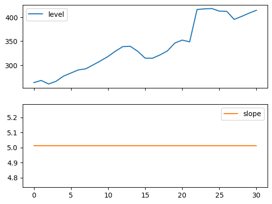
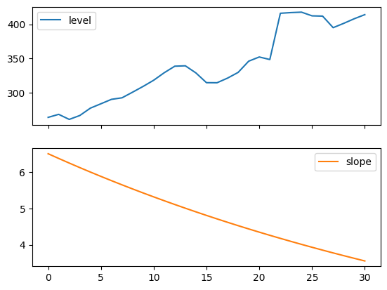
../../../_images/examples_notebooks_generated_exponential_smoothing_12_0.png

../../../_images/examples_notebooks_generated_exponential_smoothing_12_1.png

Figure 7.4: Level and slope components for Holt’s linear trend method and the additive damped trend method.

比較¶

ここでは、単純指数平滑法とホルト法を、さまざまな加法的、指数的、および減衰型の組み合わせについて比較したプロットを示します。すべてのモデルのパラメータは、statsmodelsによって最適化されます。

[7]:

fit1 = SimpleExpSmoothing(livestock2, initialization_method="estimated").fit()
fcast1 = fit1.forecast(9).rename("SES")
fit2 = Holt(livestock2, initialization_method="estimated").fit()
fcast2 = fit2.forecast(9).rename("Holt's")
fit3 = Holt(livestock2, exponential=True, initialization_method="estimated").fit()
fcast3 = fit3.forecast(9).rename("Exponential")
fit4 = Holt(livestock2, damped_trend=True, initialization_method="estimated").fit(
    damping_trend=0.98
)
fcast4 = fit4.forecast(9).rename("Additive Damped")
fit5 = Holt(
    livestock2, exponential=True, damped_trend=True, initialization_method="estimated"
).fit()
fcast5 = fit5.forecast(9).rename("Multiplicative Damped")

ax = livestock2.plot(color="black", marker="o", figsize=(12, 8))
livestock3.plot(ax=ax, color="black", marker="o", legend=False)
fcast1.plot(ax=ax, color="red", legend=True)
fcast2.plot(ax=ax, color="green", legend=True)
fcast3.plot(ax=ax, color="blue", legend=True)
fcast4.plot(ax=ax, color="cyan", legend=True)
fcast5.plot(ax=ax, color="magenta", legend=True)
ax.set_ylabel("Livestock, sheep in Asia (millions)")
plt.show()
print(
    "Figure 7.5: Forecasting livestock, sheep in Asia: comparing forecasting performance of non-seasonal methods."
)

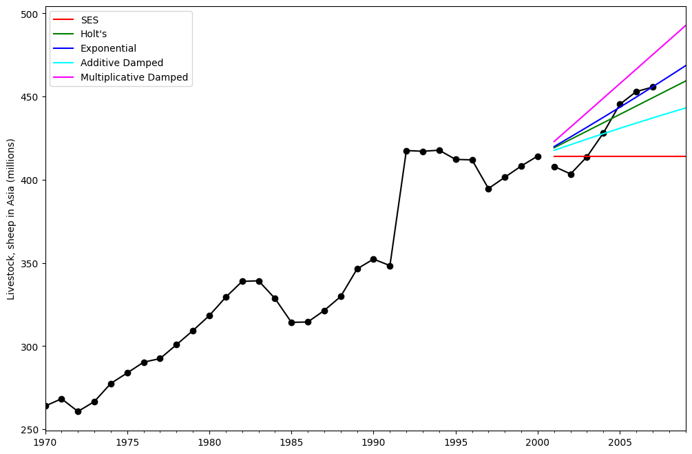
../../../_images/examples_notebooks_generated_exponential_smoothing_14_0.png

Figure 7.5: Forecasting livestock, sheep in Asia: comparing forecasting performance of non-seasonal methods.

ホルト・ウィンターズ季節指数平滑法¶

最後に、トレンド成分と季節成分を含む完全なホルト・ウィンターズ季節指数平滑法を実行できるようになります。

statsmodels は、以下に示すように、すべての組み合わせをサポートしています：

fit1 加算トレンド、加算季節（周期 season_length=4）、およびボックスコックス変換の使用。
fit2 加算トレンド、乗算季節（周期 season_length=4）、およびボックスコックス変換の使用。
fit3 加算減衰トレンド、加算季節（周期 season_length=4）、およびボックスコックス変換の使用。
fit4 加算減衰トレンド、乗算季節（周期 season_length=4）、およびボックスコックス変換の使用。

グラフは、fit1 と fit2 の結果と予測を示しています。

テーブルでは、結果とパラメータ設定を比較することができます。

[8]:

fit1 = ExponentialSmoothing(
    aust,
    seasonal_periods=4,
    trend="add",
    seasonal="add",
    use_boxcox=True,
    initialization_method="estimated",
).fit()
fit2 = ExponentialSmoothing(
    aust,
    seasonal_periods=4,
    trend="add",
    seasonal="mul",
    use_boxcox=True,
    initialization_method="estimated",
).fit()
fit3 = ExponentialSmoothing(
    aust,
    seasonal_periods=4,
    trend="add",
    seasonal="add",
    damped_trend=True,
    use_boxcox=True,
    initialization_method="estimated",
).fit()
fit4 = ExponentialSmoothing(
    aust,
    seasonal_periods=4,
    trend="add",
    seasonal="mul",
    damped_trend=True,
    use_boxcox=True,
    initialization_method="estimated",
).fit()
results = pd.DataFrame(
    index=[r"$\alpha$", r"$\beta$", r"$\phi$", r"$\gamma$", r"$l_0$", "$b_0$", "SSE"]
)
params = [
    "smoothing_level",
    "smoothing_trend",
    "damping_trend",
    "smoothing_seasonal",
    "initial_level",
    "initial_trend",
]
results["Additive"] = [fit1.params[p] for p in params] + [fit1.sse]
results["Multiplicative"] = [fit2.params[p] for p in params] + [fit2.sse]
results["Additive Dam"] = [fit3.params[p] for p in params] + [fit3.sse]
results["Multiplica Dam"] = [fit4.params[p] for p in params] + [fit4.sse]

ax = aust.plot(
    figsize=(10, 6),
    marker="o",
    color="black",
    title="Forecasts from Holt-Winters' multiplicative method",
)
ax.set_ylabel("International visitor night in Australia (millions)")
ax.set_xlabel("Year")
fit1.fittedvalues.plot(ax=ax, style="--", color="red")
fit2.fittedvalues.plot(ax=ax, style="--", color="green")

fit1.forecast(8).rename("Holt-Winters (add-add-seasonal)").plot(
    ax=ax, style="--", marker="o", color="red", legend=True
)
fit2.forecast(8).rename("Holt-Winters (add-mul-seasonal)").plot(
    ax=ax, style="--", marker="o", color="green", legend=True
)

plt.show()
print(
    "Figure 7.6: Forecasting international visitor nights in Australia using Holt-Winters method with both additive and multiplicative seasonality."
)

results

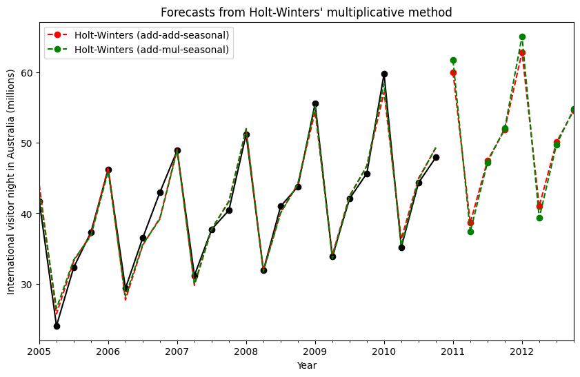
../../../_images/examples_notebooks_generated_exponential_smoothing_16_0.png

Figure 7.6: Forecasting international visitor nights in Australia using Holt-Winters method with both additive and multiplicative seasonality.

[8]:

	Additive	Multiplicative	Additive Dam	Multiplica Dam
$\alpha$	1.490116e-08	1.490116e-08	1.490116e-08	1.490116e-08
$\beta$	1.409867e-08	0.000000e+00	6.490718e-09	5.042207e-09
$\phi$	NaN	NaN	9.430416e-01	9.536043e-01
$\gamma$	0.000000e+00	0.000000e+00	0.000000e+00	0.000000e+00
$l_0$	1.119348e+01	1.106378e+01	1.084022e+01	9.899298e+00
$b_0$	1.205396e-01	1.198959e-01	2.456749e-01	1.975447e-01
SSE	4.402746e+01	3.611262e+01	3.527620e+01	3.062033e+01

モデル内部の詳細¶

指数平滑法モデルの内部にアクセスすることが可能です。

ここでは、元の値 $y_t$、レベル $l_t$、傾向 $b_t$、季節成分 $s_t$、および適合値 $\hat{y}_t$ を並べて表示できるテーブルを示します。これらの値は、Box-Cox変換を行わずにフィットを実行した場合のみ、元のデータ空間内で意味のある値を持つことに注意してください。

[9]:

fit1 = ExponentialSmoothing(
    aust,
    seasonal_periods=4,
    trend="add",
    seasonal="add",
    initialization_method="estimated",
).fit()
fit2 = ExponentialSmoothing(
    aust,
    seasonal_periods=4,
    trend="add",
    seasonal="mul",
    initialization_method="estimated",
).fit()

[10]:

df = pd.DataFrame(
    np.c_[aust, fit1.level, fit1.trend, fit1.season, fit1.fittedvalues],
    columns=[r"$y_t$", r"$l_t$", r"$b_t$", r"$s_t$", r"$\hat{y}_t$"],
    index=aust.index,
)
forecasts = fit1.forecast(8).rename(r"$\hat{y}_t$").to_frame()
df = pd.concat([df, forecasts], axis=0, sort=True)

[11]:

df = pd.DataFrame(
    np.c_[aust, fit2.level, fit2.trend, fit2.season, fit2.fittedvalues],
    columns=[r"$y_t$", r"$l_t$", r"$b_t$", r"$s_t$", r"$\hat{y}_t$"],
    index=aust.index,
)
forecasts = fit2.forecast(8).rename(r"$\hat{y}_t$").to_frame()
df = pd.concat([df, forecasts], axis=0, sort=True)

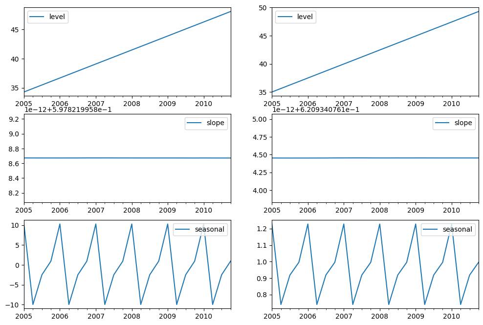
最後に、モデルのレベル、傾き/トレンド、および季節的な成分を見てみましょう。

[12]:

states1 = pd.DataFrame(
    np.c_[fit1.level, fit1.trend, fit1.season],
    columns=["level", "slope", "seasonal"],
    index=aust.index,
)
states2 = pd.DataFrame(
    np.c_[fit2.level, fit2.trend, fit2.season],
    columns=["level", "slope", "seasonal"],
    index=aust.index,
)
fig, [[ax1, ax4], [ax2, ax5], [ax3, ax6]] = plt.subplots(3, 2, figsize=(12, 8))
states1[["level"]].plot(ax=ax1)
states1[["slope"]].plot(ax=ax2)
states1[["seasonal"]].plot(ax=ax3)
states2[["level"]].plot(ax=ax4)
states2[["slope"]].plot(ax=ax5)
states2[["seasonal"]].plot(ax=ax6)
plt.show()

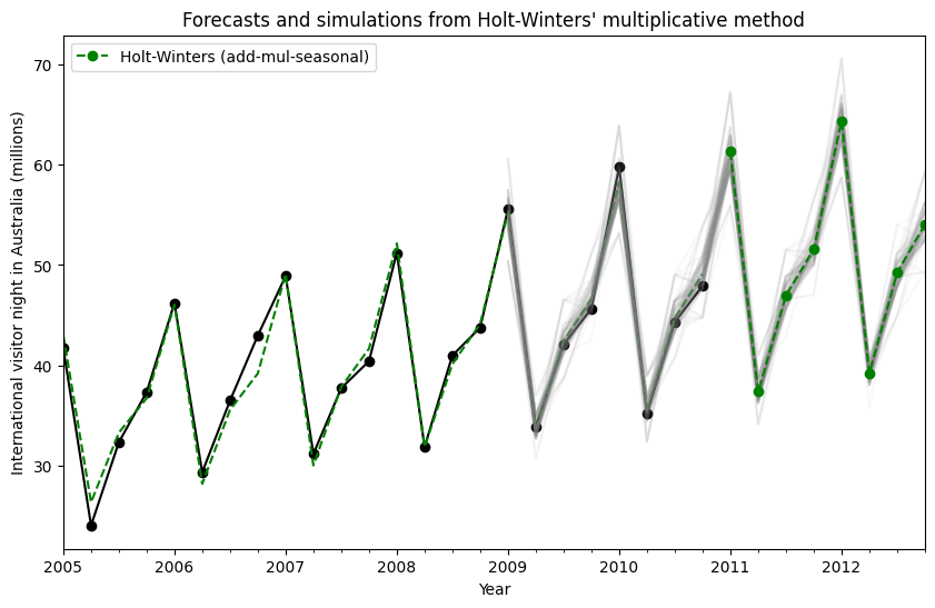
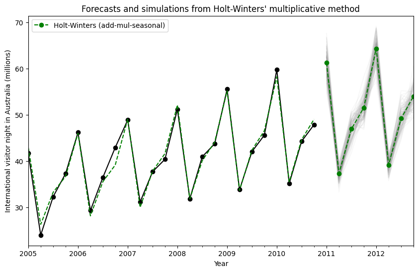
../../../_images/examples_notebooks_generated_exponential_smoothing_22_0.png

状態空間モデルを使用することにより、将来の値のシミュレーションを行うことができます。数学的な詳細については、HyndmanとAthanasopoulos [2] および HoltWintersResults.simulate のドキュメントに記載されています。

[2] の例と同様に、加法的トレンド、乗法的季節性、乗法的誤差を持つモデルを使用します。最大8ステップ先までシミュレーションを行い、1000回のシミュレーションを実施します。以下の図に示されているように、シミュレーションは予測値と非常によく一致しています。

[2] Hyndman, Rob J., and George Athanasopoulos. Forecasting: principles and practice, 2nd edition. OTexts, 2018.

[13]:

fit = ExponentialSmoothing(
    aust,
    seasonal_periods=4,
    trend="add",
    seasonal="mul",
    initialization_method="estimated",
).fit()
simulations = fit.simulate(8, repetitions=100, error="mul")

ax = aust.plot(
    figsize=(10, 6),
    marker="o",
    color="black",
    title="Forecasts and simulations from Holt-Winters' multiplicative method",
)
ax.set_ylabel("International visitor night in Australia (millions)")
ax.set_xlabel("Year")
fit.fittedvalues.plot(ax=ax, style="--", color="green")
simulations.plot(ax=ax, style="-", alpha=0.05, color="grey", legend=False)
fit.forecast(8).rename("Holt-Winters (add-mul-seasonal)").plot(
    ax=ax, style="--", marker="o", color="green", legend=True
)
plt.show()

../../../_images/examples_notebooks_generated_exponential_smoothing_24_0.png

シミュレーションは異なる時点から開始することもでき、ランダムノイズを選択するための複数のオプションがあります。

[14]:

fit = ExponentialSmoothing(
    aust,
    seasonal_periods=4,
    trend="add",
    seasonal="mul",
    initialization_method="estimated",
).fit()
simulations = fit.simulate(
    16, anchor="2009-01-01", repetitions=100, error="mul", random_errors="bootstrap"
)

ax = aust.plot(
    figsize=(10, 6),
    marker="o",
    color="black",
    title="Forecasts and simulations from Holt-Winters' multiplicative method",
)
ax.set_ylabel("International visitor night in Australia (millions)")
ax.set_xlabel("Year")
fit.fittedvalues.plot(ax=ax, style="--", color="green")
simulations.plot(ax=ax, style="-", alpha=0.05, color="grey", legend=False)
fit.forecast(8).rename("Holt-Winters (add-mul-seasonal)").plot(
    ax=ax, style="--", marker="o", color="green", legend=True
)
plt.show()

../../../_images/examples_notebooks_generated_exponential_smoothing_26_0.png

最終更新日: 2025年01月28日