ETSモデル
ETSモデルは、レベル成分、トレンド成分(T)、季節成分(S)、および誤差項(E)からなる基盤となる状態空間モデルを持つ時系列モデルの一群です。
このノートブックでは、statsmodelsを使用してこれらのモデルがどのように活用できるかを示します。より詳細な解説については、[1]の第8章(無料オンラインリソース)を参照してください。これは、statsmodelsでの実装と、このノートブックで使用される例に基づいています。
statsmodelsは、以下の全ての組み合わせを実装しています:
加法的および乗法的誤差モデル
加法的および乗法的トレンド(減衰する可能性あり)
加法的および乗法的季節性
ただし、これらの方法がすべて安定しているわけではありません。モデルの安定性に関する詳細は[1]およびその中の参考文献を参照してください。
[1] Hyndman, Rob J., と Athanasopoulos, George. Forecasting: principles and practice(第3版)、OTexts、2021年。 https://otexts.com/fpp3/expsmooth.html
[1]:
import numpy as np
import matplotlib.pyplot as plt
import pandas as pd

%matplotlib inline
from statsmodels.tsa.exponential_smoothing.ets import ETSModel
[2]:
plt.rcParams["figure.figsize"] = (12, 8)
単純指数平滑法
最も単純なETSモデルは、単純指数平滑法としても知られています。ETSの用語では、これは(A, N, N)モデルに相当します。つまり、加法的な誤差、トレンドなし、季節性なしのモデルです。Holt法の状態空間形式は次のようになります:
\begin{align} y_{t} &= y_{t-1} + e_t\\ l_{t} &= l_{t-1} + \alpha e_t\\ \end{align}
この状態空間形式は、異なる形式、予測式と平滑化式に変換できます(これはすべてのETSモデルに共通です):
\begin{align} \hat{y}_{t|t-1} &= l_{t-1}\\ l_{t} &= \alpha y_{t-1} + (1 - \alpha) l_{t-1} \end{align}
ここで、\(\hat{y}_{t|t-1}\)は前のステップの情報に基づいた\(y_t\)の予測/期待値です。単純指数平滑法モデルでは、予測は前のレベルに対応します。第二の式(平滑化式)は、次のレベルを前のレベルと前の観測値の加重平均として計算します。
[3]:
oildata = [
111.0091,
130.8284,
141.2871,
154.2278,
162.7409,
192.1665,
240.7997,
304.2174,
384.0046,
429.6622,
359.3169,
437.2519,
468.4008,
424.4353,
487.9794,
509.8284,
506.3473,
340.1842,
240.2589,
219.0328,
172.0747,
252.5901,
221.0711,
276.5188,
271.1480,
342.6186,
428.3558,
442.3946,
432.7851,
437.2497,
437.2092,
445.3641,
453.1950,
454.4096,
422.3789,
456.0371,
440.3866,
425.1944,
486.2052,
500.4291,
521.2759,
508.9476,
488.8889,
509.8706,
456.7229,
473.8166,
525.9509,
549.8338,
542.3405,
]
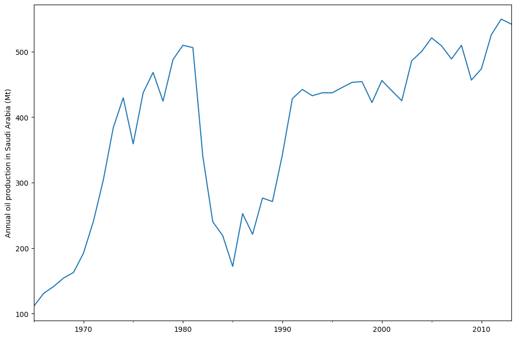
oil = pd.Series(oildata, index=pd.date_range("1965", "2013", freq="AS"))
oil.plot()
plt.ylabel("Annual oil production in Saudi Arabia (Mt)")
C:\Users\user\AppData\Local\Temp\ipykernel_17952\3897473195.py:52: FutureWarning: 'AS' is deprecated and will be removed in a future version, please use 'YS' instead.
  oil = pd.Series(oildata, index=pd.date_range("1965", "2013", freq="AS"))
[3]:
Text(0, 0.5, 'Annual oil production in Saudi Arabia (Mt)')
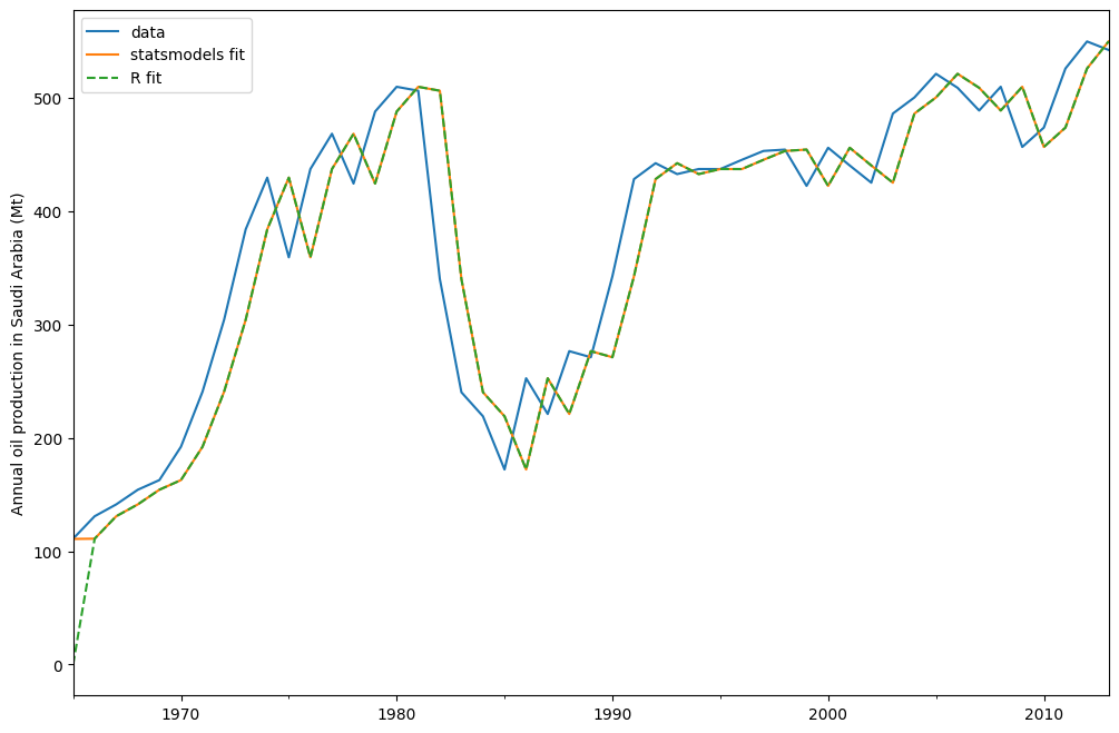
fpp2 から取得されたもので、以前のバージョン[1]の関連パッケージです。forecastを使用したフィット結果も表示されています。[4]:
model = ETSModel(oil)
fit = model.fit(maxiter=10000)
oil.plot(label="data")
fit.fittedvalues.plot(label="statsmodels fit")
plt.ylabel("Annual oil production in Saudi Arabia (Mt)")

# obtained from R
params_R = [0.99989969, 0.11888177503085334, 0.80000197, 36.46466837, 34.72584983]
yhat = model.smooth(params_R).fittedvalues
yhat.plot(label="R fit", linestyle="--")

plt.legend()
[4]:
<matplotlib.legend.Legend at 0x208820d03d0>
デフォルトでは、初期状態はフィッティングパラメータとして扱われ、対数尤度の最大化によって推定されます。初期値にはヒューリスティックな手法のみを使用することも可能です。
[5]:
model_heuristic = ETSModel(oil, initialization_method="heuristic")
fit_heuristic = model_heuristic.fit()
oil.plot(label="data")
fit.fittedvalues.plot(label="estimated")
fit_heuristic.fittedvalues.plot(label="heuristic", linestyle="--")
plt.ylabel("Annual oil production in Saudi Arabia (Mt)")

# obtained from R
params = [0.99989969, 0.11888177503085334, 0.80000197, 36.46466837, 34.72584983]
yhat = model.smooth(params).fittedvalues
yhat.plot(label="with R params", linestyle=":")

plt.legend()
[5]:
<matplotlib.legend.Legend at 0x20882184160>
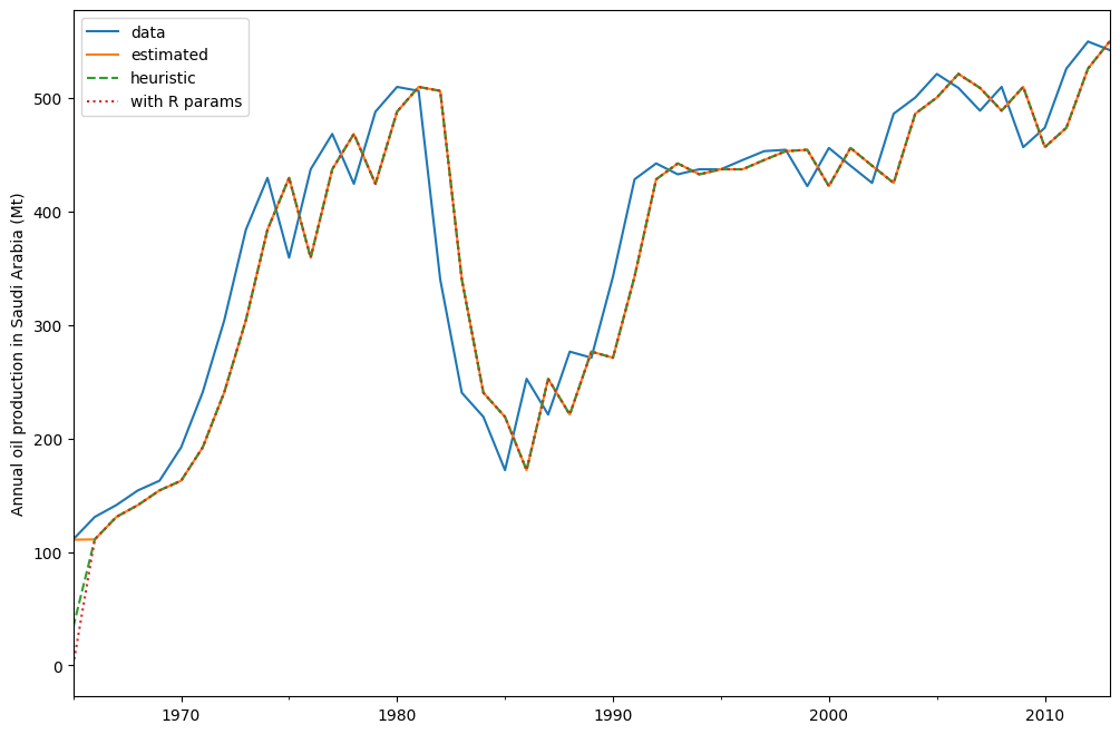
フィットしたパラメータとその他の指標は fit.summary() を使って表示されます。ここでは、初期状態にヒューリスティックを使用したモデルの対数尤度が、フィットした初期状態を使用したモデルのものよりもわずかに低いことが確認できます。
[6]:
print(fit.summary())
                                 ETS Results
==============================================================================
Dep. Variable:                      y   No. Observations:                   49
Model:                       ETS(ANN)   Log Likelihood                -259.257
Date:                Thu, 28 Nov 2024   AIC                            524.514
Time:                        23:10:29   BIC                            530.189
Sample:                    01-01-1965   HQIC                           526.667
                         - 01-01-2013   Scale                         2307.767
Covariance Type:               approx
===================================================================================
                      coef    std err          z      P>|z|      [0.025      0.975]
-----------------------------------------------------------------------------------
smoothing_level     0.9999      0.132      7.551      0.000       0.740       1.259
initial_level     110.7864     48.110      2.303      0.021      16.492     205.081
===================================================================================
Ljung-Box (Q):                        1.87   Jarque-Bera (JB):                20.78
Prob(Q):                              0.39   Prob(JB):                         0.00
Heteroskedasticity (H):               0.49   Skew:                            -1.04
Prob(H) (two-sided):                  0.16   Kurtosis:                         5.42
===================================================================================

Warnings:
[1] Covariance matrix calculated using numerical (complex-step) differentiation.
[7]:
print(fit_heuristic.summary())
                                 ETS Results
==============================================================================
Dep. Variable:                      y   No. Observations:                   49
Model:                       ETS(ANN)   Log Likelihood                -260.521
Date:                Thu, 28 Nov 2024   AIC                            525.042
Time:                        23:10:29   BIC                            528.826
Sample:                    01-01-1965   HQIC                           526.477
                         - 01-01-2013   Scale                         2429.964
Covariance Type:               approx
===================================================================================
                      coef    std err          z      P>|z|      [0.025      0.975]
-----------------------------------------------------------------------------------
smoothing_level     0.9999      0.132      7.559      0.000       0.741       1.259
==============================================
              initialization method: heuristic
----------------------------------------------
initial_level                          33.6309
===================================================================================
Ljung-Box (Q):                        1.85   Jarque-Bera (JB):                18.42
Prob(Q):                              0.40   Prob(JB):                         0.00
Heteroskedasticity (H):               0.44   Skew:                            -1.02
Prob(H) (two-sided):                  0.11   Kurtosis:                         5.21
===================================================================================

Warnings:
[1] Covariance matrix calculated using numerical (complex-step) differentiation.
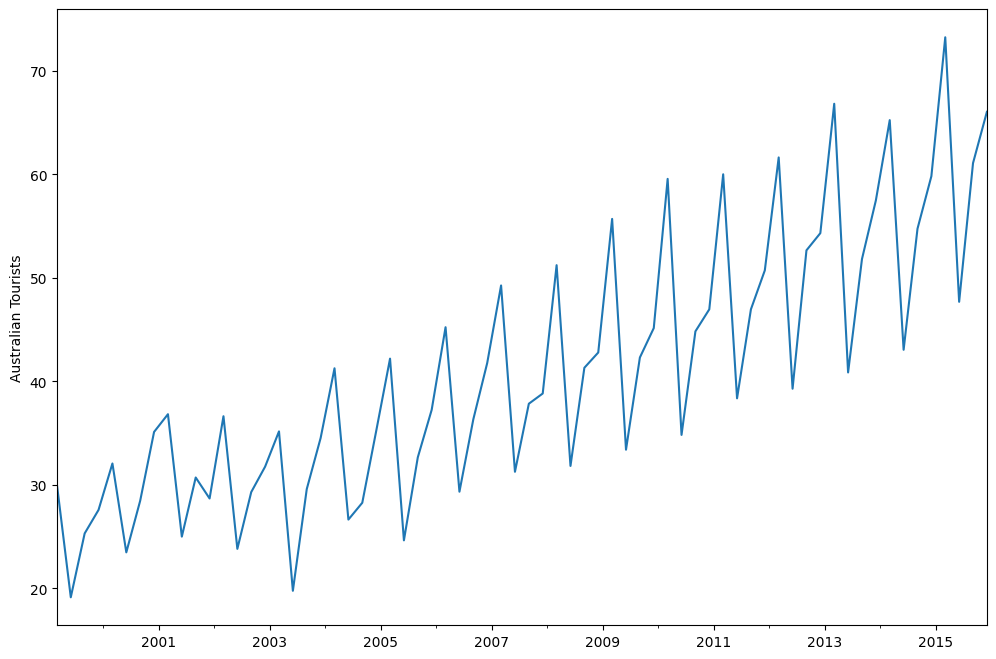
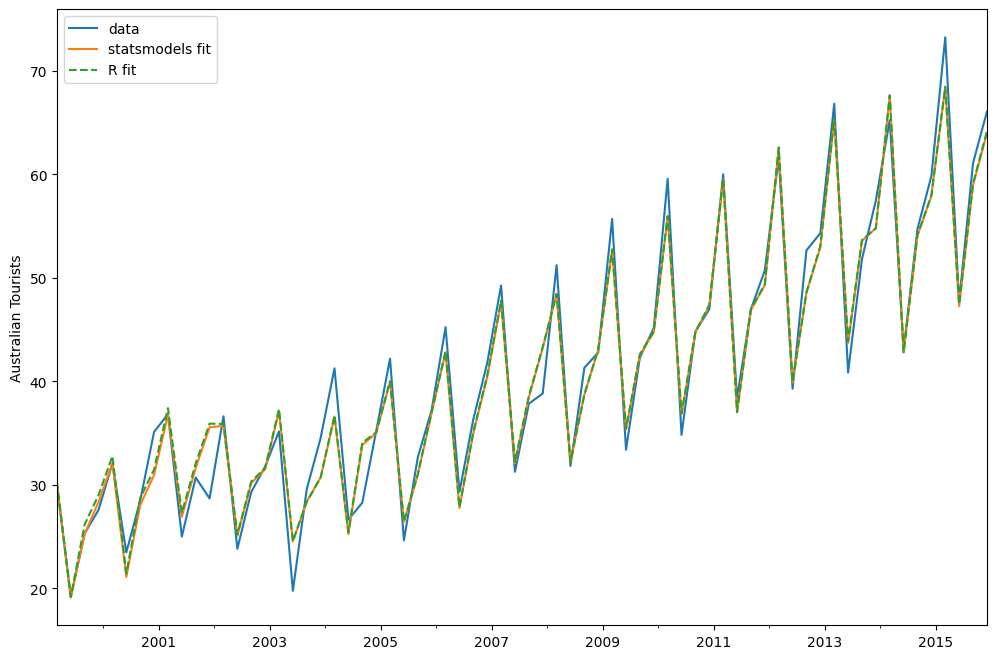
ホルト・ウィンターズの季節変動法
指数平滑法は、トレンド成分と季節成分を組み込むように修正できます。加法的ホルト・ウィンターズ法では、季節成分が残りの部分に加えられます。このモデルはETS(A, A, A)モデルに対応し、次の状態空間の定式化を持ちます:
\begin{align} y_t &= l_{t-1} + b_{t-1} + s_{t-m} + e_t\\ l_{t} &= l_{t-1} + b_{t-1} + \alpha e_t\\ b_{t} &= b_{t-1} + \beta e_t\\ s_{t} &= s_{t-m} + \gamma e_t \end{align}
[8]:
austourists_data = [
    30.05251300,
    19.14849600,
    25.31769200,
    27.59143700,
    32.07645600,
    23.48796100,
    28.47594000,
    35.12375300,
    36.83848500,
    25.00701700,
    30.72223000,
    28.69375900,
    36.64098600,
    23.82460900,
    29.31168300,
    31.77030900,
    35.17787700,
    19.77524400,
    29.60175000,
    34.53884200,
    41.27359900,
    26.65586200,
    28.27985900,
    35.19115300,
    42.20566386,
    24.64917133,
    32.66733514,
    37.25735401,
    45.24246027,
    29.35048127,
    36.34420728,
    41.78208136,
    49.27659843,
    31.27540139,
    37.85062549,
    38.83704413,
    51.23690034,
    31.83855162,
    41.32342126,
    42.79900337,
    55.70835836,
    33.40714492,
    42.31663797,
    45.15712257,
    59.57607996,
    34.83733016,
    44.84168072,
    46.97124960,
    60.01903094,
    38.37117851,
    46.97586413,
    50.73379646,
    61.64687319,
    39.29956937,
    52.67120908,
    54.33231689,
    66.83435838,
    40.87118847,
    51.82853579,
    57.49190993,
    65.25146985,
    43.06120822,
    54.76075713,
    59.83447494,
    73.25702747,
    47.69662373,
    61.09776802,
    66.05576122,
]
index = pd.date_range("1999-03-01", "2015-12-01", freq="3MS")
austourists = pd.Series(austourists_data, index=index)
austourists.plot()
plt.ylabel("Australian Tourists")
[8]:
Text(0, 0.5, 'Australian Tourists')
[9]:
# fit in statsmodels
model = ETSModel(
    austourists,
    error="add",
    trend="add",
    seasonal="add",
    damped_trend=True,
    seasonal_periods=4,
)
fit = model.fit()

# fit with R params
params_R = [
    0.35445427,
    0.03200749,
    0.39993387,
    0.97999997,
    24.01278357,
    0.97770147,
    1.76951063,
    -0.50735902,
    -6.61171798,
    5.34956637,
]
fit_R = model.smooth(params_R)

austourists.plot(label="data")
plt.ylabel("Australian Tourists")

fit.fittedvalues.plot(label="statsmodels fit")
fit_R.fittedvalues.plot(label="R fit", linestyle="--")
plt.legend()
[9]:
<matplotlib.legend.Legend at 0x208860548b0>
[10]:
print(fit.summary())
                                 ETS Results
==============================================================================
Dep. Variable:                      y   No. Observations:                   68
Model:                      ETS(AAdA)   Log Likelihood                -152.627
Date:                Thu, 28 Nov 2024   AIC                            327.254
Time:                        23:10:30   BIC                            351.668
Sample:                    03-01-1999   HQIC                           336.928
                         - 12-01-2015   Scale                            5.213
Covariance Type:               approx
======================================================================================
                         coef    std err          z      P>|z|      [0.025      0.975]
--------------------------------------------------------------------------------------
smoothing_level        0.3399      0.111      3.070      0.002       0.123       0.557
smoothing_trend        0.0259      0.008      3.154      0.002       0.010       0.042
smoothing_seasonal     0.4010      0.080      5.041      0.000       0.245       0.557
damping_trend          0.9800        nan        nan        nan         nan         nan
initial_level         29.4409   4.74e+04      0.001      1.000   -9.28e+04    9.29e+04
initial_trend          0.6147      0.392      1.567      0.117      -0.154       1.383
initial_seasonal.0    -3.4320   4.74e+04  -7.24e-05      1.000   -9.29e+04    9.28e+04
initial_seasonal.1    -5.9481   4.74e+04     -0.000      1.000   -9.29e+04    9.28e+04
initial_seasonal.2   -11.4855   4.74e+04     -0.000      1.000   -9.29e+04    9.28e+04
initial_seasonal.3          0   4.74e+04          0      1.000   -9.28e+04    9.28e+04
===================================================================================
Ljung-Box (Q):                        5.76   Jarque-Bera (JB):                 7.70
Prob(Q):                              0.67   Prob(JB):                         0.02
Heteroskedasticity (H):               0.46   Skew:                            -0.63
Prob(H) (two-sided):                  0.07   Kurtosis:                         4.05
===================================================================================

Warnings:
[1] Covariance matrix calculated using numerical (complex-step) differentiation.
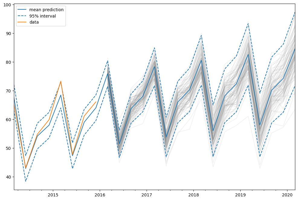
予測
ETSモデルは予測にも使用できます。いくつかの異なる方法があります:
forecast: 標本外の予測を行うpredict: 標本内および標本外の予測を行うsimulate: 状態空間モデルのシミュレーションを実行するget_prediction: 標本内および標本外の予測を行い、予測区間も提供する
これらを以前に適合させたモデルに使用して、2014年から2020年までの予測を行うことができます。
[11]:
pred = fit.get_prediction(start="2014", end="2020")
[12]:
df = pred.summary_frame(alpha=0.05)
df
[12]:
| mean | pi_lower | pi_upper | |
|---|---|---|---|
| 2014-03-01 | 67.610926 | 63.135953 | 72.085899 |
| 2014-06-01 | 42.814534 | 38.339561 | 47.289507 |
| 2014-09-01 | 54.106399 | 49.631426 | 58.581372 |
| 2014-12-01 | 57.928232 | 53.453259 | 62.403204 |
| 2015-03-01 | 68.422037 | 63.947064 | 72.897010 |
| 2015-06-01 | 47.278132 | 42.803159 | 51.753105 |
| 2015-09-01 | 58.954911 | 54.479938 | 63.429884 |
| 2015-12-01 | 63.982281 | 59.507308 | 68.457254 |
| 2016-03-01 | 75.905266 | 71.430293 | 80.380239 |
| 2016-06-01 | 51.417926 | 46.653727 | 56.182125 |
| 2016-09-01 | 63.703065 | 58.628997 | 68.777133 |
| 2016-12-01 | 67.977755 | 62.575199 | 73.380311 |
| 2017-03-01 | 78.315246 | 71.735000 | 84.895491 |
| 2017-06-01 | 53.779706 | 46.882508 | 60.676903 |
| 2017-09-01 | 66.017609 | 58.787255 | 73.247964 |
| 2017-12-01 | 70.246008 | 62.667652 | 77.824364 |
| 2018-03-01 | 80.538134 | 71.891483 | 89.184785 |
| 2018-06-01 | 55.958136 | 46.966880 | 64.949392 |
| 2018-09-01 | 68.152471 | 58.803847 | 77.501095 |
| 2018-12-01 | 72.338173 | 62.620421 | 82.055925 |
| 2019-03-01 | 82.588455 | 71.863153 | 93.313757 |
| 2019-06-01 | 57.967451 | 46.874297 | 69.060605 |
| 2019-09-01 | 70.121600 | 58.650477 | 81.592722 |
| 2019-12-01 | 74.267919 | 62.409479 | 86.126358 |
| 2020-03-01 | 84.479606 | 71.654614 | 97.304598 |
この場合、予測区間は解析的な式を使用して計算されました。これはすべてのモデルで利用できるわけではありません。その他のモデルでは、予測区間は複数回のシミュレーション(デフォルトで1000回)を実行し、シミュレーション結果のパーセンタイルを使用して計算されます。これは get_prediction メソッドによって内部で実行されます。
また、シミュレーションを手動で実行することもできます。例えば、それらをプロットするためです。データが2015年末まであるため、2016年第1四半期から2020年第1四半期までシミュレーションを行う必要があり、これは17ステップを意味します。
[13]:
simulated = fit.simulate(anchor="end", nsimulations=17, repetitions=100)
[14]:
for i in range(simulated.shape[1]):
    simulated.iloc[:, i].plot(label="_", color="gray", alpha=0.1)
df["mean"].plot(label="mean prediction")
df["pi_lower"].plot(linestyle="--", color="tab:blue", label="95% interval")
df["pi_upper"].plot(linestyle="--", color="tab:blue", label="_")
pred.endog.plot(label="data")
plt.legend()
[14]:
<matplotlib.legend.Legend at 0x20885bc2740>
この場合、シミュレーションのアンカーとして「end」を選択しました。これは、最初のシミュレートされた値が最初の標本外の値になることを意味します。標本内の他の位置をアンカーとして選択することも可能です。