状態空間モデルにおけるパラメータの推定または指定
このノートブックでは、statsmodelsの状態空間モデルにおいて、いくつかのパラメータを推定しながら、特定のパラメータの値を固定する方法を示します。
一般に、状態空間モデルでは、ユーザーは次のことができます:
すべてのパラメータを最尤推定によって推定する
一部のパラメータを固定し、残りを推定する
すべてのパラメータを固定する(つまり、パラメータは推定されない)
[1]:
%matplotlib inline

from importlib import reload
import numpy as np
import pandas as pd
import statsmodels.api as sm
import matplotlib.pyplot as plt

from pandas_datareader.data import DataReader
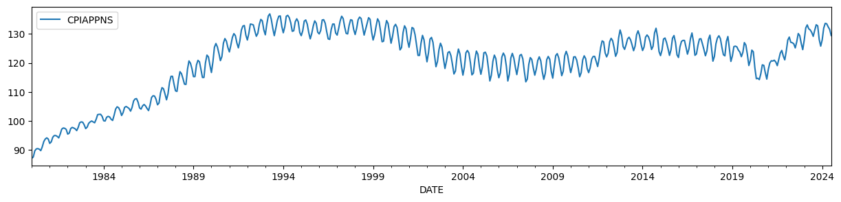
例を示すために、時間的に変動するレベルと強い季節的要素を持つ衣料品の消費者物価指数を使用します。
[2]:
endog = DataReader('CPIAPPNS', 'fred', start='1980').asfreq('MS')
endog.plot(figsize=(15, 3));
次のように翻訳できます:
HPフィルターの出力は、パラメータに関する特定の制約が与えられた場合、未観測成分モデルによって生成できることはよく知られています(例:Harvey and Jaeger [1993])。
未観測成分モデルは次のようになります:
トレンドがHPフィルターの出力と一致するためには、パラメータは次のように設定する必要があります:
ここで、\(\lambda\)は関連するHPフィルターのパラメータです。ここで使用する月次データの場合、通常、\(\lambda = 129600\)が推奨されます。
[3]:
# Run the HP filter with lambda = 129600
hp_cycle, hp_trend = sm.tsa.filters.hpfilter(endog, lamb=129600)

# The unobserved components model above is the local linear trend, or "lltrend", specification
mod = sm.tsa.UnobservedComponents(endog, 'lltrend')
print(mod.param_names)
['sigma2.irregular', 'sigma2.level', 'sigma2.trend']
未観測成分モデル(UCM)のパラメータは以下のように記述されます:
\(\sigma_\varepsilon^2 = \text{sigma2.irregular}\)
\(\sigma_\eta^2 = \text{sigma2.level}\)
\(\sigma_\zeta^2 = \text{sigma2.trend}\)
上記の制約を満たすために、\((\sigma_\varepsilon^2, \sigma_\eta^2, \sigma_\zeta^2) = (1, 0, 1 / 129600)\)と設定します。
ここではすべてのパラメータを固定しているため、最尤推定を実行するためにfitメソッドを使用する必要はありません。代わりに、選択したパラメータを使用してカルマンフィルタとスムーザーを直接実行することができます。smoothメソッドを使用して行います。
[4]:
res = mod.smooth([1., 0, 1. / 129600])
print(res.summary())
                        Unobserved Components Results
==============================================================================
Dep. Variable:               CPIAPPNS   No. Observations:                  535
Model:             local linear trend   Log Likelihood               -2996.247
Date:                Wed, 28 Aug 2024   AIC                           5998.495
Time:                        14:39:34   BIC                           6011.330
Sample:                    01-01-1980   HQIC                          6003.518
                         - 07-01-2024
Covariance Type:                  opg
====================================================================================
                       coef    std err          z      P>|z|      [0.025      0.975]
------------------------------------------------------------------------------------
sigma2.irregular     1.0000      0.009    115.613      0.000       0.983       1.017
sigma2.level              0      0.000          0      1.000      -0.000       0.000
sigma2.trend      7.716e-06   1.98e-07     38.958      0.000    7.33e-06     8.1e-06
===================================================================================
Ljung-Box (L1) (Q):                 253.96   Jarque-Bera (JB):                 1.64
Prob(Q):                              0.00   Prob(JB):                         0.44
Heteroskedasticity (H):               2.23   Skew:                             0.04
Prob(H) (two-sided):                  0.00   Kurtosis:                         2.74
===================================================================================

Warnings:
[1] Covariance matrix calculated using the outer product of gradients (complex-step).
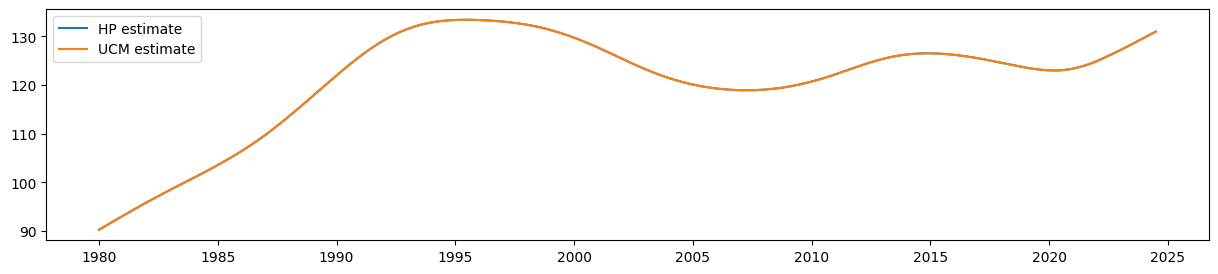
HPフィルターのトレンド推定に対応する推定値は、level(上記の記法では\(\mu_t\))の平滑化された推定値によって与えられます。
[5]:
ucm_trend = pd.Series(res.level.smoothed, index=endog.index)
UCMからの平滑化されたレベルの推定値が、HPフィルターの出力と等しいことは簡単にわかります。
[6]:
fig, ax = plt.subplots(figsize=(15, 3))

ax.plot(hp_trend, label='HP estimate')
ax.plot(ucm_trend, label='UCM estimate')
ax.legend();
季節成分を追加する
しかし、未観測成分モデルはHPフィルタよりも柔軟です。例えば、上に示したデータは明らかに季節性がありますが、時間変動する季節効果を持っています(季節性は初めの方が終わりよりもかなり弱いです)。未観測成分フレームワークの利点の一つは、確率的季節成分を追加できる点です。この場合、最尤法で季節成分の分散を推定し、上記で示唆されたパラメータに対する制約を含めて、トレンドがHPフィルタの概念に対応するようにします。
確率的季節成分を追加することで、新たに1つのパラメータ「sigma2.seasonal」が追加されます。
[7]:
# Construct a local linear trend model with a stochastic seasonal component of period 1 year
mod = sm.tsa.UnobservedComponents(endog, 'lltrend', seasonal=12, stochastic_seasonal=True)
print(mod.param_names)
['sigma2.irregular', 'sigma2.level', 'sigma2.trend', 'sigma2.seasonal']
この場合、前述のように最初の3つのパラメータを引き続き制約を加えますが、sigma2.seasonalの値を最尤推定によって推定したいと考えています。したがって、fitメソッドとともにfix_paramsコンテキストマネージャを使用します。
fix_paramsメソッドは、パラメータ名と関連する値の辞書を受け取ります。生成されたコンテキスト内では、それらのパラメータはすべてのケースで使用されます。fitメソッドの場合、固定されたパラメータ以外のパラメータのみが推定されます。
[8]:
# Here we restrict the first three parameters to specific values
with mod.fix_params({'sigma2.irregular': 1, 'sigma2.level': 0, 'sigma2.trend': 1. / 129600}):
    # Now we fit any remaining parameters, which in this case
    # is just `sigma2.seasonal`
    res_restricted = mod.fit()
代わりに、制約の辞書も受け入れるfit_constrainedメソッドを単純に使用することもできました。
[9]:
res_restricted = mod.fit_constrained({'sigma2.irregular': 1, 'sigma2.level': 0, 'sigma2.trend': 1. / 129600})
サマリー出力にはすべてのパラメータが含まれていますが、最初の3つは固定されていたため(推定されていません)、その旨が示されています。
[10]:
print(res_restricted.summary())
                            Unobserved Components Results
=====================================================================================
Dep. Variable:                      CPIAPPNS   No. Observations:                  535
Model:                    local linear trend   Log Likelihood               -1745.075
                   + stochastic seasonal(12)   AIC                           3492.150
Date:                       Wed, 28 Aug 2024   BIC                           3496.408
Time:                               14:39:35   HQIC                          3493.818
Sample:                           01-01-1980
                                - 07-01-2024
Covariance Type:                         opg
============================================================================================
                               coef    std err          z      P>|z|      [0.025      0.975]
--------------------------------------------------------------------------------------------
sigma2.irregular (fixed)     1.0000        nan        nan        nan         nan         nan
sigma2.level (fixed)              0        nan        nan        nan         nan         nan
sigma2.trend (fixed)      7.716e-06        nan        nan        nan         nan         nan
sigma2.seasonal              0.0917      0.007     12.677      0.000       0.078       0.106
===================================================================================
Ljung-Box (L1) (Q):                 458.78   Jarque-Bera (JB):                38.39
Prob(Q):                              0.00   Prob(JB):                         0.00
Heteroskedasticity (H):               2.44   Skew:                             0.30
Prob(H) (two-sided):                  0.00   Kurtosis:                         4.18
===================================================================================

Warnings:
[1] Covariance matrix calculated using the outer product of gradients (complex-step).
比較のために、制約のない最尤推定(MLE)を構築します。この場合、レベルの推定値はもはやHPフィルターの概念に対応しなくなります。
[11]:
res_unrestricted = mod.fit()
最後に、トレンドおよび季節成分の平滑化された推定値を取得できます。
[12]:
# Construct the smoothed level estimates
unrestricted_trend = pd.Series(res_unrestricted.level.smoothed, index=endog.index)
restricted_trend = pd.Series(res_restricted.level.smoothed, index=endog.index)

# Construct the smoothed estimates of the seasonal pattern
unrestricted_seasonal = pd.Series(res_unrestricted.seasonal.smoothed, index=endog.index)
restricted_seasonal = pd.Series(res_restricted.seasonal.smoothed, index=endog.index)
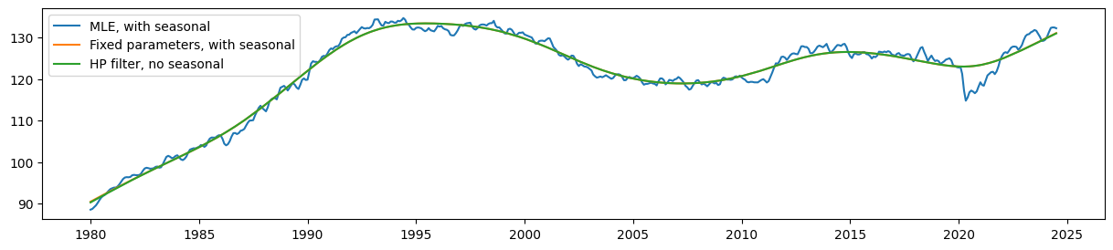
推定されたレベルを比較すると、固定パラメータを持つ季節性UCMが依然としてHPフィルターの出力に非常に近い(ただし、もはや完全に一致するわけではない)トレンドを生成していることが明らかです。
一方、パラメータ制約のないモデル(最尤推定モデル)から得られた推定レベルは、これらに比べてはるかに滑らかさに欠けています。
[13]:
fig, ax = plt.subplots(figsize=(15, 3))

ax.plot(unrestricted_trend, label='MLE, with seasonal')
ax.plot(restricted_trend, label='Fixed parameters, with seasonal')
ax.plot(hp_trend, label='HP filter, no seasonal')
ax.legend();
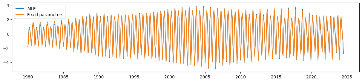
最後に、パラメータ制約を持つUCMは、時間変動する季節成分を非常にうまく捉えることができます。
[14]:
fig, ax = plt.subplots(figsize=(15, 3))

ax.plot(unrestricted_seasonal, label='MLE')
ax.plot(restricted_seasonal, label='Fixed parameters')
ax.legend();