時系列データにおける季節性
異なる周期性を持つ複数の季節成分を含む時系列データのモデリング問題を考えます。時系列データ ( y_t ) を取り、レベル成分と2つの季節成分に明示的に分解するとします。
ここで、\(\mu_t\) はトレンドまたはレベルを表し、\(\gamma^{(1)}_t\) は比較的短い周期を持つ季節成分を表し、\(\gamma^{(2)}_t\) はより長い周期を持つ別の季節成分を表します。レベルには固定の切片項を持たせ、\(\gamma^{(1)}_t\) と \(\gamma^{(2)}_t\) の両方を確率的なものとみなし、時間とともに季節パターンが変化するように考慮します。
このノートブックでは、このモデルに準拠した合成データを生成し、未観測成分モデリングフレームワークの下で季節項をいくつか異なる方法でモデリングする例を示します。
[1]:
%matplotlib inline
[2]:
import numpy as np
import pandas as pd
import statsmodels.api as sm
import matplotlib.pyplot as plt

plt.rc("figure", figsize=(16,8))
plt.rc("font", size=14)
合成データの作成
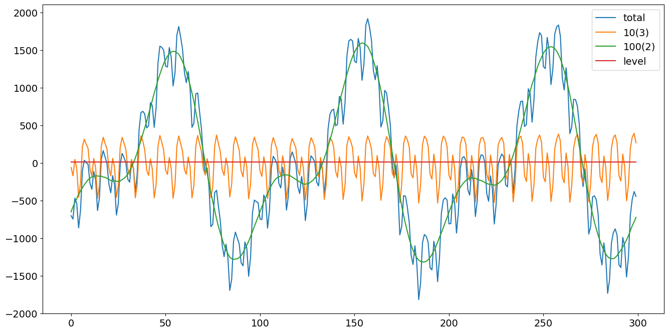
Durbin and Koopman (2012) の式 (3.7) および (3.8) に従い、複数の季節パターンを持つデータを作成します。300期間をシミュレーションし、周波数領域でパラメータ化された2つの季節項を導入します。それぞれの周期は 10 と 100 で、調和数はそれぞれ 3 と2 です。さらに、それらの確率的部分の分散はそれぞれ4と9とします。
[3]:
# First we'll simulate the synthetic data
def simulate_seasonal_term(periodicity, total_cycles, noise_std=1.,
                           harmonics=None):
    duration = periodicity * total_cycles
    assert duration == int(duration)
    duration = int(duration)
    harmonics = harmonics if harmonics else int(np.floor(periodicity / 2))

    lambda_p = 2 * np.pi / float(periodicity)

    gamma_jt = noise_std * np.random.randn((harmonics))
    gamma_star_jt = noise_std * np.random.randn((harmonics))

    total_timesteps = 100 * duration # Pad for burn in
    series = np.zeros(total_timesteps)
    for t in range(total_timesteps):
        gamma_jtp1 = np.zeros_like(gamma_jt)
        gamma_star_jtp1 = np.zeros_like(gamma_star_jt)
        for j in range(1, harmonics + 1):
            cos_j = np.cos(lambda_p * j)
            sin_j = np.sin(lambda_p * j)
            gamma_jtp1[j - 1] = (gamma_jt[j - 1] * cos_j
                                 + gamma_star_jt[j - 1] * sin_j
                                 + noise_std * np.random.randn())
            gamma_star_jtp1[j - 1] = (- gamma_jt[j - 1] * sin_j
                                      + gamma_star_jt[j - 1] * cos_j
                                      + noise_std * np.random.randn())
        series[t] = np.sum(gamma_jtp1)
        gamma_jt = gamma_jtp1
        gamma_star_jt = gamma_star_jtp1
    wanted_series = series[-duration:] # Discard burn in

    return wanted_series
[4]:
duration = 100 * 3
periodicities = [10, 100]
num_harmonics = [3, 2]
std = np.array([2, 3])
np.random.seed(8678309)

terms = []
for ix, _ in enumerate(periodicities):
    s = simulate_seasonal_term(
        periodicities[ix],
        duration / periodicities[ix],
        harmonics=num_harmonics[ix],
        noise_std=std[ix])
    terms.append(s)
terms.append(np.ones_like(terms[0]) * 10.)
series = pd.Series(np.sum(terms, axis=0))
df = pd.DataFrame(data={'total': series,
                        '10(3)': terms[0],
                        '100(2)': terms[1],
                        'level':terms[2]})
h1, = plt.plot(df['total'])
h2, = plt.plot(df['10(3)'])
h3, = plt.plot(df['100(2)'])
h4, = plt.plot(df['level'])
plt.legend(['total','10(3)','100(2)', 'level'])
plt.show()
未観測成分(周波数領域モデリング)
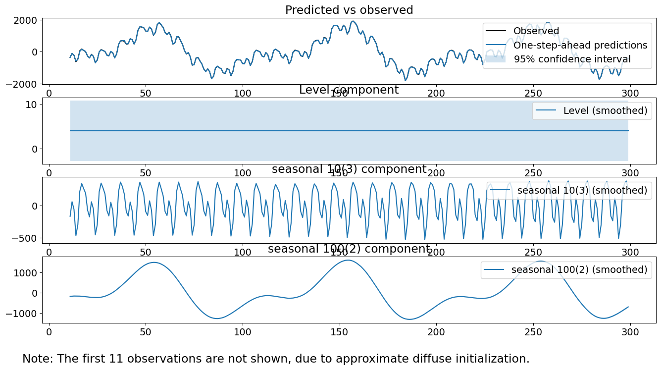
次に示す方法は未観測成分モデルであり、トレンドは固定された切片としてモデル化され、季節性成分は主周期がそれぞれ10と100の三角関数を用いてモデル化されます。それぞれの高調波の数は3と2です。このモデルは生成モデルとして正しいものです。時系列の過程は以下のように書けます:
ここで、\(\epsilon_t\)はホワイトノイズ、\(\omega^{(1)}_{j,t}\)は独立同分布の\(N(0, \sigma^2_1)\)、\(\omega^{(2)}_{j,t}\)は独立同分布の\(N(0, \sigma^2_2)\)であり、\(\sigma_1 = 2\)です。
[5]:
model = sm.tsa.UnobservedComponents(series.values,
                                    level='fixed intercept',
                                    freq_seasonal=[{'period': 10,
                                                    'harmonics': 3},
                                                   {'period': 100,
                                                    'harmonics': 2}])
res_f = model.fit(disp=False)
print(res_f.summary())
# The first state variable holds our estimate of the intercept
print("fixed intercept estimated as {0:.3f}".format(res_f.smoother_results.smoothed_state[0,-1:][0]))

res_f.plot_components()
plt.show()
                                Unobserved Components Results
==============================================================================================
Dep. Variable:                                      y   No. Observations:                  300
Model:                                fixed intercept   Log Likelihood               -1145.631
                    + stochastic freq_seasonal(10(3))   AIC                           2295.261
                   + stochastic freq_seasonal(100(2))   BIC                           2302.594
Date:                                Wed, 28 Aug 2024   HQIC                          2298.200
Time:                                        15:01:24
Sample:                                             0
                                                - 300
Covariance Type:                                  opg
===============================================================================================
                                  coef    std err          z      P>|z|      [0.025      0.975]
-----------------------------------------------------------------------------------------------
sigma2.freq_seasonal_10(3)      4.5942      0.565      8.126      0.000       3.486       5.702
sigma2.freq_seasonal_100(2)     9.7904      2.483      3.942      0.000       4.923      14.658
===================================================================================
Ljung-Box (L1) (Q):                   0.06   Jarque-Bera (JB):                 0.08
Prob(Q):                              0.81   Prob(JB):                         0.96
Heteroskedasticity (H):               1.17   Skew:                             0.01
Prob(H) (two-sided):                  0.45   Kurtosis:                         3.08
===================================================================================

Warnings:
[1] Covariance matrix calculated using the outer product of gradients (complex-step).
fixed intercept estimated as 4.053
[6]:
model.ssm.transition[:, :, 0]
[6]:
array([[ 1.        ,  0.        ,  0.        ,  0.        ,  0.        ,
         0.        ,  0.        ,  0.        ,  0.        ,  0.        ,
         0.        ],
       [ 0.        ,  0.80901699,  0.58778525,  0.        ,  0.        ,
         0.        ,  0.        ,  0.        ,  0.        ,  0.        ,
         0.        ],
       [ 0.        , -0.58778525,  0.80901699,  0.        ,  0.        ,
         0.        ,  0.        ,  0.        ,  0.        ,  0.        ,
         0.        ],
       [ 0.        ,  0.        ,  0.        ,  0.30901699,  0.95105652,
         0.        ,  0.        ,  0.        ,  0.        ,  0.        ,
         0.        ],
       [ 0.        ,  0.        ,  0.        , -0.95105652,  0.30901699,
         0.        ,  0.        ,  0.        ,  0.        ,  0.        ,
         0.        ],
       [ 0.        ,  0.        ,  0.        ,  0.        ,  0.        ,
        -0.30901699,  0.95105652,  0.        ,  0.        ,  0.        ,
         0.        ],
       [ 0.        ,  0.        ,  0.        ,  0.        ,  0.        ,
        -0.95105652, -0.30901699,  0.        ,  0.        ,  0.        ,
         0.        ],
       [ 0.        ,  0.        ,  0.        ,  0.        ,  0.        ,
         0.        ,  0.        ,  0.99802673,  0.06279052,  0.        ,
         0.        ],
       [ 0.        ,  0.        ,  0.        ,  0.        ,  0.        ,
         0.        ,  0.        , -0.06279052,  0.99802673,  0.        ,
         0.        ],
       [ 0.        ,  0.        ,  0.        ,  0.        ,  0.        ,
         0.        ,  0.        ,  0.        ,  0.        ,  0.9921147 ,
         0.12533323],
       [ 0.        ,  0.        ,  0.        ,  0.        ,  0.        ,
         0.        ,  0.        ,  0.        ,  0.        , -0.12533323,
         0.9921147 ]])
適合された分散は、真の分散である4と9にかなり近いことが確認できます。さらに、個々の季節成分も真の季節成分に非常に近いように見えます。平滑化されたレベル項も、真のレベルである10にある程度近いです。最後に、診断結果は良好であり、3つの検定のいずれも棄却されない程度に検定統計量が小さいことが確認できます。
未観測成分(時間および周波数領域の混合モデリング)
2つ目の方法は、観測されない要素モデルです。このモデルでは、トレンドを固定された切片としてモデル化し、季節成分を0に和がなる10個の定数と、周期性が100で2つの高調波を含む三角関数を使用してモデル化します。ただし、このモデルは生成モデルではありません。というのも、より短い季節成分に対して現実よりも多くの状態誤差が存在することを前提としているからです。時系列のプロセスは以下のように書くことができます:
ここで、\(\epsilon_t\)はホワイトノイズであり、\(\omega^{(1)}_{t}\)は独立同分布の\(N(0, \sigma^2_1)\)に従い、\(\omega^{(2)}_{j,t}\)は独立同分布の\(N(0, \sigma^2_2)\)に従います。
[7]:
model = sm.tsa.UnobservedComponents(series,
                                    level='fixed intercept',
                                    seasonal=10,
                                    freq_seasonal=[{'period': 100,
                                                    'harmonics': 2}])
res_tf = model.fit(disp=False)
print(res_tf.summary())
# The first state variable holds our estimate of the intercept
print("fixed intercept estimated as {0:.3f}".format(res_tf.smoother_results.smoothed_state[0,-1:][0]))

fig = res_tf.plot_components()
fig.tight_layout(pad=1.0)
                                Unobserved Components Results
==============================================================================================
Dep. Variable:                                      y   No. Observations:                  300
Model:                                fixed intercept   Log Likelihood               -1238.113
                            + stochastic seasonal(10)   AIC                           2480.226
                   + stochastic freq_seasonal(100(2))   BIC                           2487.538
Date:                                Wed, 28 Aug 2024   HQIC                          2483.157
Time:                                        15:01:25
Sample:                                             0
                                                - 300
Covariance Type:                                  opg
===============================================================================================
                                  coef    std err          z      P>|z|      [0.025      0.975]
-----------------------------------------------------------------------------------------------
sigma2.seasonal                55.2934      7.114      7.773      0.000      41.351      69.236
sigma2.freq_seasonal_100(2)    28.6897      4.008      7.159      0.000      20.835      36.544
===================================================================================
Ljung-Box (L1) (Q):                  26.35   Jarque-Bera (JB):                 1.20
Prob(Q):                              0.00   Prob(JB):                         0.55
Heteroskedasticity (H):               1.27   Skew:                            -0.14
Prob(H) (two-sided):                  0.24   Kurtosis:                         2.87
===================================================================================

Warnings:
[1] Covariance matrix calculated using the outer product of gradients (complex-step).
fixed intercept estimated as 4.468
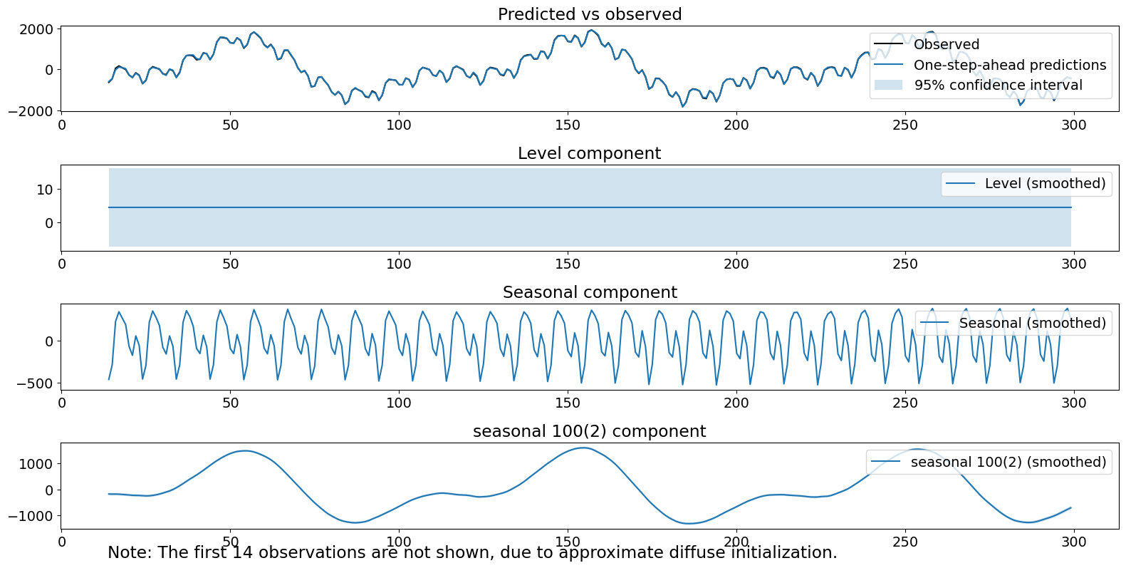
プロットされた成分は良好に見えます。ただし、第二の季節項の推定分散は実際よりも膨らんでいます。さらに、Ljung-Box統計量を棄却しており、成分を考慮した後でも残存する自己相関がある可能性を示唆しています。
未観測成分(遅延周波数領域モデル)
第三の方法は、固定された切片と1つの季節成分を持つ観測されない成分モデルで、これは主要な周期性が100、50の高調波を持つ三角関数を使ってモデル化されます。これは生成モデルではないことに注意してください。実際には高調波がそれより少ないため、このモデルはより多くの高調波があることを前提としています。分散が一緒に結びついているため、存在しない高調波の推定共分散を0にすることができません。このモデル仕様が怠惰である理由は、2つの異なる季節成分を指定することを省略し、代わりに両方をカバーするのに十分な高調波を持つ単一の成分を使用してモデル化したことです。これにより、2つの真の成分間の分散の違いを捉えることはできません。この時系列のプロセスは次のように書くことができます:
ここで、\(\epsilon_t\)はホワイトノイズ、\(\omega^{(1)}_{t}\)は独立同分布で\(N(0, \sigma^2_1)\)です。
[8]:
model = sm.tsa.UnobservedComponents(series,
                                    level='fixed intercept',
                                    freq_seasonal=[{'period': 100}])
res_lf = model.fit(disp=False)
print(res_lf.summary())
# The first state variable holds our estimate of the intercept
print("fixed intercept estimated as {0:.3f}".format(res_lf.smoother_results.smoothed_state[0,-1:][0]))

fig = res_lf.plot_components()
fig.tight_layout(pad=1.0)
                                 Unobserved Components Results
===============================================================================================
Dep. Variable:                                       y   No. Observations:                  300
Model:                                 fixed intercept   Log Likelihood               -1101.455
                   + stochastic freq_seasonal(100(50))   AIC                           2204.910
Date:                                 Wed, 28 Aug 2024   BIC                           2208.204
Time:                                         15:01:34   HQIC                          2206.243
Sample:                                              0
                                                 - 300
Covariance Type:                                   opg
================================================================================================
                                   coef    std err          z      P>|z|      [0.025      0.975]
------------------------------------------------------------------------------------------------
sigma2.freq_seasonal_100(50)     0.7591      0.082      9.233      0.000       0.598       0.920
===================================================================================
Ljung-Box (L1) (Q):                  85.96   Jarque-Bera (JB):                 0.72
Prob(Q):                              0.00   Prob(JB):                         0.70
Heteroskedasticity (H):               1.00   Skew:                            -0.01
Prob(H) (two-sided):                  0.99   Kurtosis:                         2.71
===================================================================================

Warnings:
[1] Covariance matrix calculated using the outer product of gradients (complex-step).
fixed intercept estimated as 4.426
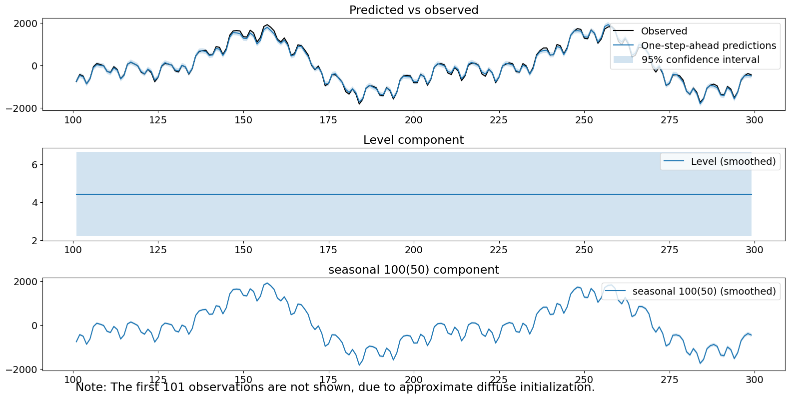
私たちの診断テストのうち、1つは0.05の有意水準で棄却されることに注意してください。
未観測測成分(遅延時間領域季節モデリング)
第四の方法は、固定された切片と、100個の定数を用いた時間領域季節モデルで表現された単一の季節成分を持つ観測されない成分モデルです。時系列のプロセスは次のように表すことができます:
ここで、\(\epsilon_t\) はホワイトノイズ、\(\omega^{(1)}_{t}\) は独立同分布の \(N(0, \sigma^2_1)\) です。
[9]:
model = sm.tsa.UnobservedComponents(series,
                                    level='fixed intercept',
                                    seasonal=100)
res_lt = model.fit(disp=False)
print(res_lt.summary())
# The first state variable holds our estimate of the intercept
print("fixed intercept estimated as {0:.3f}".format(res_lt.smoother_results.smoothed_state[0,-1:][0]))

fig = res_lt.plot_components()
fig.tight_layout(pad=1.0)
                            Unobserved Components Results
======================================================================================
Dep. Variable:                              y   No. Observations:                  300
Model:                        fixed intercept   Log Likelihood               -1564.378
                   + stochastic seasonal(100)   AIC                           3130.756
Date:                        Wed, 28 Aug 2024   BIC                           3134.054
Time:                                15:01:43   HQIC                          3132.091
Sample:                                     0
                                        - 300
Covariance Type:                          opg
===================================================================================
                      coef    std err          z      P>|z|      [0.025      0.975]
-----------------------------------------------------------------------------------
sigma2.seasonal  3.558e+05   2.96e+04     12.012      0.000    2.98e+05    4.14e+05
===================================================================================
Ljung-Box (L1) (Q):                 200.79   Jarque-Bera (JB):                25.29
Prob(Q):                              0.00   Prob(JB):                         0.00
Heteroskedasticity (H):               0.49   Skew:                             0.85
Prob(H) (two-sided):                  0.00   Kurtosis:                         3.37
===================================================================================

Warnings:
[1] Covariance matrix calculated using the outer product of gradients (complex-step).
fixed intercept estimated as 4.690
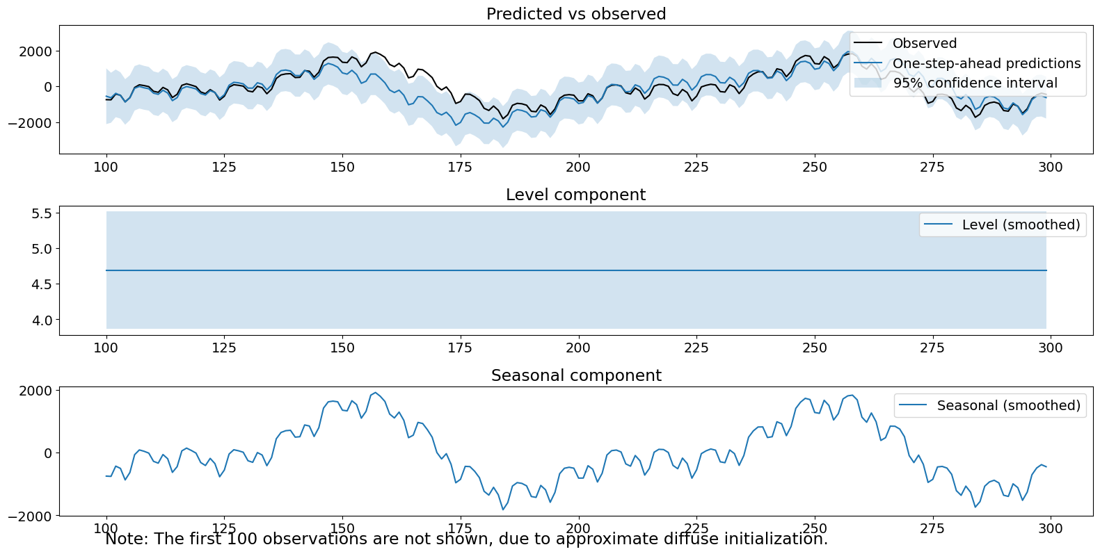
季節成分自体は良好で、主要な信号となっています。季節項の推定分散は非常に高く(\(>10^5\))、そのため、1ステップ先の予測における不確実性が大きく、また新しいデータに対する反応が遅くなっています。これは、1ステップ先の予測と観測で大きな誤差が見られることで確認できます。最後に、私たちの診断テスト3つすべてが棄却されました。
フィルタ推定の比較
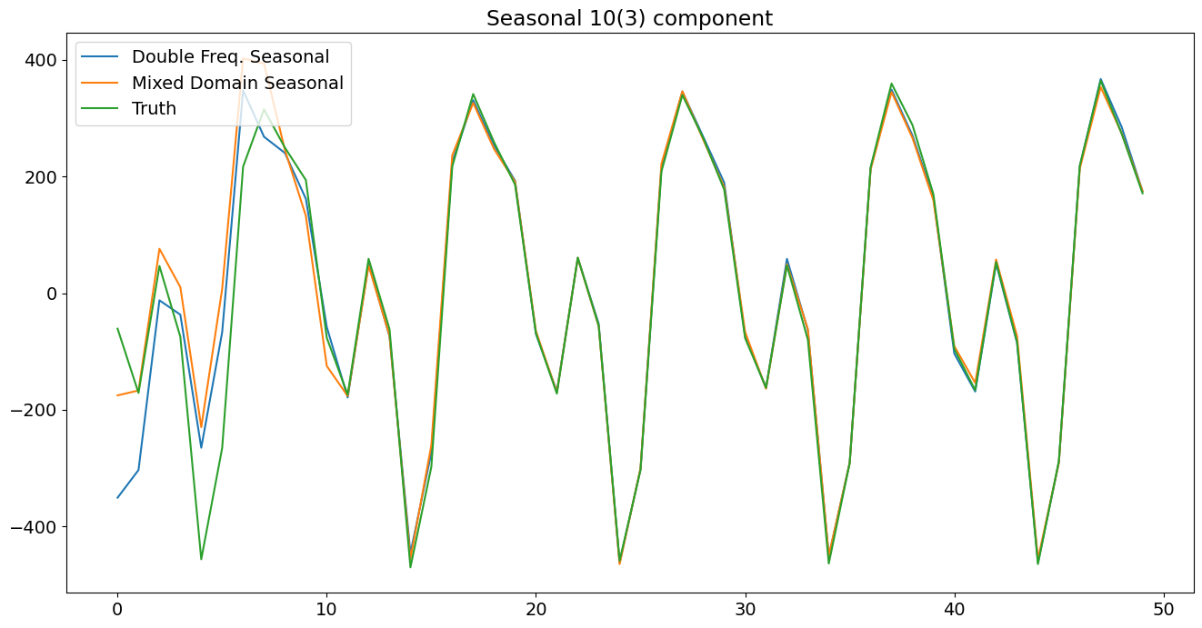
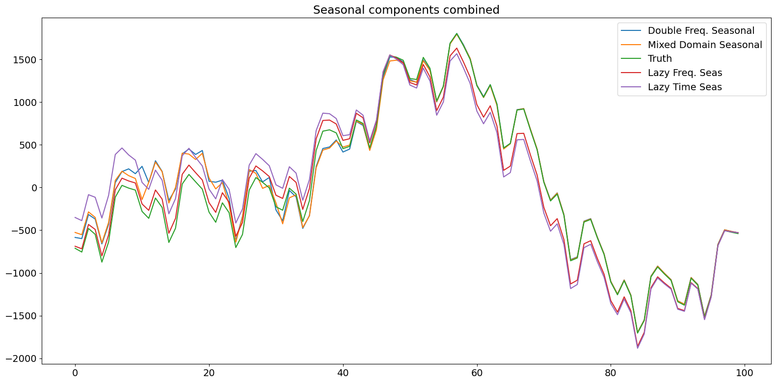
以下のプロットは、個々の成分を明示的にモデル化することで、フィルタリングされた状態が真の状態にほぼ半周期以内で近づくことを示しています。一方、遅延モデルは、結合された真の状態に対して同じことを行うのにより長い時間(ほぼ1周期)を要しました。
[10]:
# Assign better names for our seasonal terms
true_seasonal_10_3 = terms[0]
true_seasonal_100_2 = terms[1]
true_sum = true_seasonal_10_3 + true_seasonal_100_2
[11]:
time_s = np.s_[:50]  # After this they basically agree
fig1 = plt.figure()
ax1 = fig1.add_subplot(111)
idx = np.asarray(series.index)
h1, = ax1.plot(idx[time_s], res_f.freq_seasonal[0].filtered[time_s], label='Double Freq. Seas')
h2, = ax1.plot(idx[time_s], res_tf.seasonal.filtered[time_s], label='Mixed Domain Seas')
h3, = ax1.plot(idx[time_s], true_seasonal_10_3[time_s], label='True Seasonal 10(3)')
plt.legend([h1, h2, h3], ['Double Freq. Seasonal','Mixed Domain Seasonal','Truth'], loc=2)
plt.title('Seasonal 10(3) component')
plt.show()
[12]:
time_s = np.s_[:50] # After this they basically agree
fig2 = plt.figure()
ax2 = fig2.add_subplot(111)
h21, = ax2.plot(idx[time_s], res_f.freq_seasonal[1].filtered[time_s], label='Double Freq. Seas')
h22, = ax2.plot(idx[time_s], res_tf.freq_seasonal[0].filtered[time_s], label='Mixed Domain Seas')
h23, = ax2.plot(idx[time_s], true_seasonal_100_2[time_s], label='True Seasonal 100(2)')
plt.legend([h21, h22, h23], ['Double Freq. Seasonal','Mixed Domain Seasonal','Truth'], loc=2)
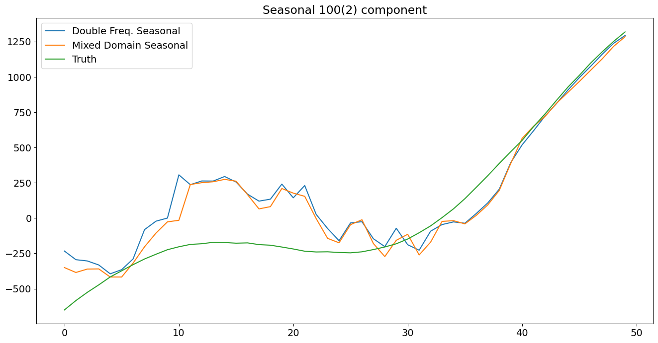
plt.title('Seasonal 100(2) component')
plt.show()
[13]:
time_s = np.s_[:100]

fig3 = plt.figure()
ax3 = fig3.add_subplot(111)
h31, = ax3.plot(idx[time_s], res_f.freq_seasonal[1].filtered[time_s] + res_f.freq_seasonal[0].filtered[time_s], label='Double Freq. Seas')
h32, = ax3.plot(idx[time_s], res_tf.freq_seasonal[0].filtered[time_s] + res_tf.seasonal.filtered[time_s], label='Mixed Domain Seas')
h33, = ax3.plot(idx[time_s], true_sum[time_s], label='True Seasonal 100(2)')
h34, = ax3.plot(idx[time_s], res_lf.freq_seasonal[0].filtered[time_s], label='Lazy Freq. Seas')
h35, = ax3.plot(idx[time_s], res_lt.seasonal.filtered[time_s], label='Lazy Time Seas')

plt.legend([h31, h32, h33, h34, h35], ['Double Freq. Seasonal','Mixed Domain Seasonal','Truth', 'Lazy Freq. Seas', 'Lazy Time Seas'], loc=1)
plt.title('Seasonal components combined')
plt.tight_layout(pad=1.0)
結論
このノートブックでは、異なる期間の2つの季節的な成分を持つ時系列をシミュレートしました。それらを以下のように構造的時系列モデルでモデル化しました:(a)正しい期間と調和数を持つ2つの周波数領域成分、(b)短期の時間領域季節成分と正しい期間と調和数を持つ周波数領域成分、(c)長い期間を持つ単一の周波数領域成分と完全な調和数、(d)長い期間を持つ単一の時間領域成分。さまざまな診断結果が見られましたが、正しい生成モデルである(a)のみが、いずれのテストでも棄却されませんでした。したがって、調和数を指定できる複数の成分を許容する柔軟な季節モデルは、時系列モデリングにおいて有用なツールとなる可能性があります。最後に、この方法で季節成分をより少ない総状態で表現できるため、ユーザーが「怠惰な」モデルを選ばされるのではなく、バイアス-分散トレードオフを自分で試みることができるようになります。