失業率のトレンドとサイクル
ここでは、経済データにおけるトレンドとサイクルを分離するための3つの方法を考えます。時系列 \(y_t\) が与えられていると仮定し、基本的なアイデアはこれを2つの成分に分解することです:
ここで、\(\mu_t\) はトレンドまたはレベルを表し、\(\eta_t\) はサイクル成分を表します。この場合、確率的トレンドを考慮し、\(\mu_t\) はランダム変数であり、時間の決定論的関数ではないとします。3つの方法のうち2つは「未観測成分」モデルに分類され、3番目は一般的なホドリック・プレスコット(HP)フィルターです。Harvey and Jaeger(1993)などと一致するように、これらのモデルはすべて似たような分解を生成することが分かります。
このノートブックでは、これらのモデルを適用して米国の失業率におけるトレンドとサイクルを分離する方法を示します。
[1]:
%matplotlib inline
[2]:
import numpy as np
import pandas as pd
import statsmodels.api as sm
import matplotlib.pyplot as plt
[3]:
from pandas_datareader.data import DataReader
endog = DataReader('UNRATE', 'fred', start='1954-01-01')
endog.index.freq = endog.index.inferred_freq
ホドリック・プレスコット(HP)フィルター
最初の方法はホドリック・プレスコットフィルターで、これはデータ系列に非常に直感的に適用できます。ここでは、失業率が月次で観測されるため、パラメータ\(\lambda=129600\)を指定します。
[4]:
hp_cycle, hp_trend = sm.tsa.filters.hpfilter(endog, lamb=129600)
観測されない成分とARIMAモデル(UC-ARIMA)
次の方法は、観測されない成分モデルで、ここではトレンドがランダムウォークとしてモデル化され、サイクルはARIMAモデルでモデル化されます。特に、ここではAR(4)モデルを使用します。時系列のプロセスは次のように表すことができます:
ここで、\(\phi(L)\)はAR(4)のラグ多項式であり、\(\epsilon_t\)と\(\nu_t\)はホワイトノイズです。
[5]:
mod_ucarima = sm.tsa.UnobservedComponents(endog, 'rwalk', autoregressive=4)
# Here the powell method is used, since it achieves a
# higher loglikelihood than the default L-BFGS method
res_ucarima = mod_ucarima.fit(method='powell', disp=False)
print(res_ucarima.summary())
                        Unobserved Components Results
==============================================================================
Dep. Variable:                 UNRATE   No. Observations:                  847
Model:                    random walk   Log Likelihood                -463.600
                              + AR(4)   AIC                            939.201
Date:                Wed, 28 Aug 2024   BIC                            967.644
Time:                        14:38:13   HQIC                           950.099
Sample:                    01-01-1954
                         - 07-01-2024
Covariance Type:                  opg
================================================================================
                   coef    std err          z      P>|z|      [0.025      0.975]
--------------------------------------------------------------------------------
sigma2.level  6.057e-08      0.011   5.47e-06      1.000      -0.022       0.022
sigma2.ar        0.1747      0.015     11.774      0.000       0.146       0.204
ar.L1            1.0258      0.019     54.132      0.000       0.989       1.063
ar.L2           -0.1060      0.016     -6.612      0.000      -0.137      -0.075
ar.L3            0.0755      0.023      3.264      0.001       0.030       0.121
ar.L4           -0.0268      0.019     -1.422      0.155      -0.064       0.010
===================================================================================
Ljung-Box (L1) (Q):                   0.00   Jarque-Bera (JB):           6636081.73
Prob(Q):                              0.97   Prob(JB):                         0.00
Heteroskedasticity (H):               9.13   Skew:                            17.45
Prob(H) (two-sided):                  0.00   Kurtosis:                       435.48
===================================================================================

Warnings:
[1] Covariance matrix calculated using the outer product of gradients (complex-step).
確率的サイクルを持つ未観測成分モデル (UC)
最終的な方法も未観測成分モデルですが、ここではサイクルが明示的にモデル化されています。
[6]:
mod_uc = sm.tsa.UnobservedComponents(
    endog, 'rwalk',
    cycle=True, stochastic_cycle=True, damped_cycle=True,
)
# Here the powell method gets close to the optimum
res_uc = mod_uc.fit(method='powell', disp=False)
# but to get to the highest loglikelihood we do a
# second round using the L-BFGS method.
res_uc = mod_uc.fit(res_uc.params, disp=False)
print(res_uc.summary())
                            Unobserved Components Results
=====================================================================================
Dep. Variable:                        UNRATE   No. Observations:                  847
Model:                           random walk   Log Likelihood                -472.370
                   + damped stochastic cycle   AIC                            952.740
Date:                       Wed, 28 Aug 2024   BIC                            971.693
Time:                               14:38:13   HQIC                           960.002
Sample:                           01-01-1954
                                - 07-01-2024
Covariance Type:                         opg
===================================================================================
                      coef    std err          z      P>|z|      [0.025      0.975]
-----------------------------------------------------------------------------------
sigma2.level        0.0177      0.032      0.547      0.585      -0.046       0.081
sigma2.cycle        0.1546      0.032      4.866      0.000       0.092       0.217
frequency.cycle     0.0436      0.029      1.508      0.131      -0.013       0.100
damping.cycle       0.9564      0.019     51.381      0.000       0.920       0.993
===================================================================================
Ljung-Box (L1) (Q):                   1.53   Jarque-Bera (JB):           6534930.78
Prob(Q):                              0.22   Prob(JB):                         0.00
Heteroskedasticity (H):               9.48   Skew:                            17.30
Prob(H) (two-sided):                  0.00   Kurtosis:                       432.69
===================================================================================

Warnings:
[1] Covariance matrix calculated using the outer product of gradients (complex-step).
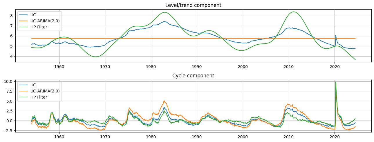
グラフィカル比較
これらの各モデルの出力は、トレンド成分 \(\mu_t\) と循環成分 \(\eta_t\) の推定値です。定性的には、トレンドとサイクルの推定値は非常に似ているものの、HPフィルターによるトレンド成分は、観測されない成分モデルによるものよりもやや変動が大きいです。これは、失業率の動きの比較的多くが一時的な循環的動きではなく、基礎的なトレンドの変化に起因していることを意味します。
[7]:
fig, axes = plt.subplots(2, figsize=(13,5));
axes[0].set(title='Level/trend component')
axes[0].plot(endog.index, res_uc.level.smoothed, label='UC')
axes[0].plot(endog.index, res_ucarima.level.smoothed, label='UC-ARIMA(2,0)')
axes[0].plot(hp_trend, label='HP Filter')
axes[0].legend(loc='upper left')
axes[0].grid()

axes[1].set(title='Cycle component')
axes[1].plot(endog.index, res_uc.cycle.smoothed, label='UC')
axes[1].plot(endog.index, res_ucarima.autoregressive.smoothed, label='UC-ARIMA(2,0)')
axes[1].plot(hp_cycle, label='HP Filter')
axes[1].legend(loc='upper left')
axes[1].grid()

fig.tight_layout();